Two Sided Expected Exceedance criterion

Description

Evaluation of a two-sided Expected Exceedance criterion. To be used in optimization routines, like in max_infill_criterion.

Usage

tsee_optim(x, model, T)

Arguments

Value

tsee criterion. When the argument x is a vector the function returns a scalar. When the argument x is a p*d matrix the function returns a vector of size p.

Author(s)

Clement Chevalier (IMSV, Switzerland, and IRSN, France) Yann Richet (IRSN, France)

See Also

EGI, max_infill_criterion

Examples

#tsee_optim

set.seed(8)
N <- 9 #number of observations
T <- 80 #threshold
testfun <- branin

#a 9 points initial design
design <- data.frame( matrix(runif(2*N),ncol=2) )
response <- testfun(design)

#km object with matern3_2 covariance
#params estimated by ML from the observations
model <- km(formula=~., design = design, 
	response = response,covtype="matern3_2")

x <- c(0.5,0.4)#one evaluation of the tsee criterion
tsee_optim(x=x,T=T,model=model)

n.grid <- 20 #you can run it with 100
x.grid <- y.grid <- seq(0,1,length=n.grid)
x <- expand.grid(x.grid, y.grid)
tsee.grid <- tsee_optim(x=x,T=T,model=model)
z.grid <- matrix(tsee.grid, n.grid, n.grid)

#plots: contour of the criterion, doe points and new point
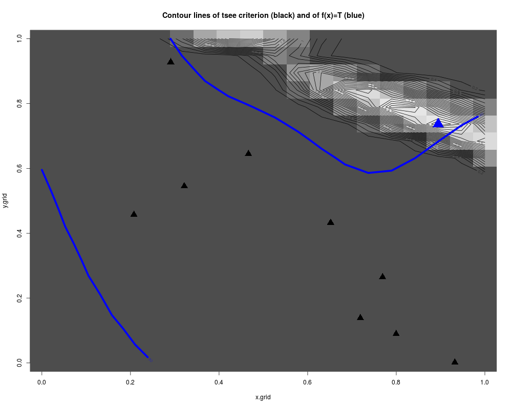
image(x=x.grid,y=y.grid,z=z.grid,col=grey.colors(10))
contour(x=x.grid,y=y.grid,z=z.grid,25,add=TRUE)
points(design, col="black", pch=17, lwd=4,cex=2)

i.best <- which.max(tsee.grid)
points(x[i.best,], col="blue", pch=17, lwd=4,cex=3)

#plots the real (unknown in practice) curve f(x)=T
testfun.grid <- apply(x,1,testfun)
z.grid.2 <- matrix(testfun.grid, n.grid, n.grid)
contour(x.grid,y.grid,z.grid.2,levels=T,col="blue",add=TRUE,lwd=5)
title("Contour lines of tsee criterion (black) and of f(x)=T (blue)")

Results

R version 3.3.1 (2016-06-21) -- "Bug in Your Hair"
Copyright (C) 2016 The R Foundation for Statistical Computing
Platform: x86_64-pc-linux-gnu (64-bit)

R is free software and comes with ABSOLUTELY NO WARRANTY.
You are welcome to redistribute it under certain conditions.
Type 'license()' or 'licence()' for distribution details.

R is a collaborative project with many contributors.
Type 'contributors()' for more information and
'citation()' on how to cite R or R packages in publications.

Type 'demo()' for some demos, 'help()' for on-line help, or
'help.start()' for an HTML browser interface to help.
Type 'q()' to quit R.

> library(KrigInv)
Loading required package: DiceKriging
Loading required package: pbivnorm
Loading required package: rgenoud
##  rgenoud (Version 5.7-12.4, Build Date: 2015-07-19)
##  See http://sekhon.berkeley.edu/rgenoud for additional documentation.
##  Please cite software as:
##   Walter Mebane, Jr. and Jasjeet S. Sekhon. 2011.
##   ``Genetic Optimization Using Derivatives: The rgenoud package for R.''
##   Journal of Statistical Software, 42(11): 1-26. 
##

Loading required package: randtoolbox
Loading required package: rngWELL
This is randtoolbox. For overview, type 'help("randtoolbox")'.
> png(filename="/home/ddbj/snapshot/RGM3/R_CC/result/KrigInv/tsee_optim.Rd_%03d_medium.png", width=480, height=480)
> ### Name: tsee_optim
> ### Title: Two Sided Expected Exceedance criterion
> ### Aliases: tsee_optim
> 
> ### ** Examples
> 
> #tsee_optim
> 
> set.seed(8)
> N <- 9 #number of observations
> T <- 80 #threshold
> testfun <- branin
> 
> #a 9 points initial design
> design <- data.frame( matrix(runif(2*N),ncol=2) )
> response <- testfun(design)
> 
> #km object with matern3_2 covariance
> #params estimated by ML from the observations
> model <- km(formula=~., design = design, 
+ 	response = response,covtype="matern3_2")

optimisation start
------------------
* estimation method   : MLE 
* optimisation method : BFGS 
* analytical gradient : used
* trend model : ~X1 + X2
* covariance model : 
  - type :  matern3_2 
  - nugget : NO
  - parameters lower bounds :  1e-10 1e-10 
  - parameters upper bounds :  1.448893 1.853021 
  - best initial criterion value(s) :  -25.38168 

N = 2, M = 5 machine precision = 2.22045e-16
At X0, 0 variables are exactly at the bounds
At iterate     0  f=       25.382  |proj g|=      0.19431
At iterate     1  f =       25.027  |proj g|=       0.13259
At iterate     2  f =       25.014  |proj g|=        1.6725
At iterate     3  f =       25.002  |proj g|=       0.15969
At iterate     4  f =       25.001  |proj g|=       0.17792
At iterate     5  f =       24.999  |proj g|=       0.31318
At iterate     6  f =       24.998  |proj g|=       0.14968
At iterate     7  f =       24.998  |proj g|=       0.03446
At iterate     8  f =       24.998  |proj g|=       0.03458
At iterate     9  f =       24.998  |proj g|=     0.0084816
At iterate    10  f =       24.998  |proj g|=      0.038393
At iterate    11  f =       24.997  |proj g|=        1.3196
At iterate    12  f =       24.997  |proj g|=        1.3327
At iterate    13  f =       24.994  |proj g|=        1.8077
At iterate    14  f =       24.991  |proj g|=        1.8106
At iterate    15  f =       24.975  |proj g|=        1.8136
At iterate    16  f =       24.937  |proj g|=        1.8202
At iterate    17  f =       24.816  |proj g|=        1.8136
At iterate    18  f =       24.652  |proj g|=       0.81261
At iterate    19  f =       24.652  |proj g|=       0.25743
At iterate    20  f =       24.651  |proj g|=     0.0033442
At iterate    21  f =       24.651  |proj g|=    1.4045e-05

iterations 21
function evaluations 30
segments explored during Cauchy searches 22
BFGS updates skipped 0
active bounds at final generalized Cauchy point 1
norm of the final projected gradient 1.40447e-05
final function value 24.6515

F = 24.6515
final  value 24.651471 
converged
> 
> x <- c(0.5,0.4)#one evaluation of the tsee criterion
> tsee_optim(x=x,T=T,model=model)
[1] 9.473495e-66
> 
> n.grid <- 20 #you can run it with 100
> x.grid <- y.grid <- seq(0,1,length=n.grid)
> x <- expand.grid(x.grid, y.grid)
> tsee.grid <- tsee_optim(x=x,T=T,model=model)
> z.grid <- matrix(tsee.grid, n.grid, n.grid)
> 
> #plots: contour of the criterion, doe points and new point
> image(x=x.grid,y=y.grid,z=z.grid,col=grey.colors(10))
> contour(x=x.grid,y=y.grid,z=z.grid,25,add=TRUE)
> points(design, col="black", pch=17, lwd=4,cex=2)
> 
> i.best <- which.max(tsee.grid)
> points(x[i.best,], col="blue", pch=17, lwd=4,cex=3)
> 
> #plots the real (unknown in practice) curve f(x)=T
> testfun.grid <- apply(x,1,testfun)
> z.grid.2 <- matrix(testfun.grid, n.grid, n.grid)
> contour(x.grid,y.grid,z.grid.2,levels=T,col="blue",add=TRUE,lwd=5)
> title("Contour lines of tsee criterion (black) and of f(x)=T (blue)")
> 
> 
> 
> 
> 
> dev.off()
null device 
          1 
>