Auto-constructing Frechet derivative of D-criterion based on general equivalence theorem

Description

Auto-constructs Frechet derivative of D-criterion at M(ξ, β) and in direction M(ξ_x, β) where M is Fisher information matrix, β is vector of parameters, ξ is the interested design and ξ_x is a unique design which has only a point x. The constructed Frechet derivative is an R function with argument x.

Usage

cfderiv(ymean, yvar, param, points, weights)

Arguments

Details

If response variables have the same constant variance, for example σ^2, then yvar must be 1.

Consider design ξ with n m-dimensional points. Then, the vector of ξ points is

(x_1, x_2, …, x_i, …, x_n),

where x_i = (x_{i1}, x_{i2}, …, x_{im}). Hence the length of vector points is mn.

Value

Note

A design ξ is D-optimal if and only if Frechet derivative at M(ξ, β) and in direction M(ξ_x, β)is greater than or equal to 0 on the design space. The equality must be achieved just at ξ points. Here, x is an arbitrary point on design space.

This function is applicable for models that can be written as E(Y_i) = f(x_i,β) where y_i is the ith response variable, x_i is the observation vector of the ith explanatory variables, β is the vector of parameters and f is a continuous and differentiable function with respect to β. In addition, response variables must be independent with distributions that belong to the Natural exponential family. Logistic,Poisson, Negative Binomial, Exponential, Richards, Weibull, Log-linear, Inverse Quadratic and Michaelis-Menten are examples of these models.

Author(s)

Ehsan Masoudi, Majid Sarmad and Hooshang Talebi

References

Masoudi, E., Sarmad, M. and Talebi, H. 2012, An Almost General Code in R to Find Optimal Design, In Proceedings of the 1st ISM International Statistical Conference 2012, 292-297.

Kiefer, J. C. 1974, General equivalence theory for optimum designs (approximate theory), Ann. Statist., 2, 849-879.7.

Examples

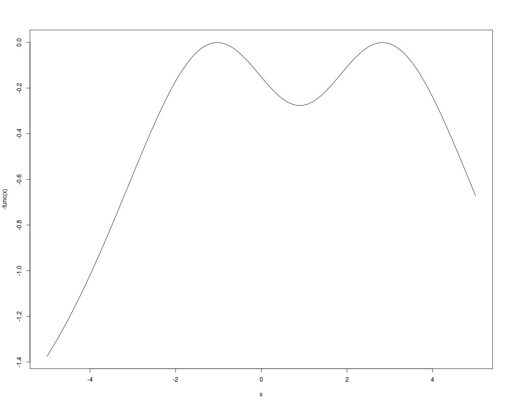
## Logistic dose response model:
ymean <- "(1/(exp(-b2 * (x1 - b1)) + 1))"
yvar <- "(1/(exp(-b2 * (x1 - b1)) + 1))*(1 - (1/(exp(-b2 * (x1 - b1)) + 1)))"
func <- cfderiv(ymean, yvar, param =  c(.9, .8), points = c(-1.029256, 2.829256),
 weights = c(.5, .5))
## plot func on the design interval to verify the optimality of the given design
x <- seq(-5, 5, by = .1)
plot(x, -func(x), type = "l")

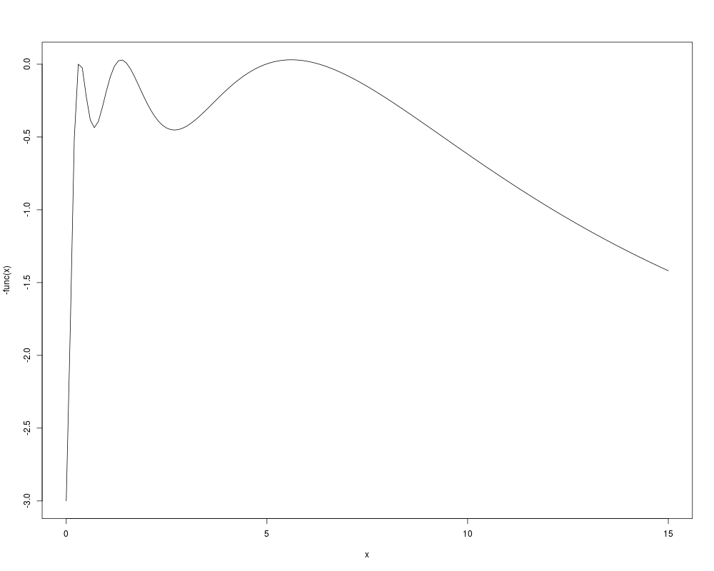
## Inverse Quadratic model
ymean <- "x1/(b1 + b2 * x1 + b3 * (x1)^2)"
yvar <- "1"
func <- cfderiv(ymean, yvar, param = c(17, 15, 9), points = c(0.33, 1.37, 5.62), 
weights = rep(.33, 3))
## plot func on the design interval to verify the optimality of the given design
x <- seq(0, 15, by = .1)
plot(x, -func(x), type = "l")

#####################################################################
## In the following, ymean and yvar for some famous models are given:

## Inverse Quadratic model (another form):
ymean <- "(b1 * x1)/(b2 + x1 + b3 * (x1)^2)"
yvar <- "1"

## Logistic dose response model:
ymean <- "(1/(exp(-b2 * (x1 - b1)) + 1))"
yvar <- "(1/(exp(-b2 * (x1 - b1)) + 1)) * (1 - (1/(exp(-b2 * (x1 - b1)) + 1)))"

## Logistic model:
ymean <- "1/(exp(-b1 - b2 * x1) + 1)"
yvar <- "(1/(exp(-b1 - b2 * x1) + 1)) * (1 - (1/(exp(-b1 - b2 * x1) + 1)))"

## Poisson model:
ymean <- yvar <-  "exp(b1 + b2 * x1)"

## Poisson dose response model:
ymean <- yvar <- "b1 * exp(-b2 * x1)"

## Weibull model:
ymean <- "b1 - b2 * exp(-b3 * x1^b4)"
yvar <- "1"

## Richards model:
ymean <- "b1/(1 + b2 * exp(-b3 * x1))^b4"
yvar <- "1"

## Michaelis-Menten model:
ymean <- "(b1 * x1)/(1 + b2 * x1)"
yvar <- "1"
#
ymean <- "(b1 * x1)/(b2 + x1)"
yvar <= "1"
#
ymean <- "x1/(b1 + b2 * x1)"
yvar <- "1"

## log-linear model:
ymean <- "b1 + b2 * log(x1 + b3)"
yvar <- "1"

## Exponential model:
ymean <- "b1 + b2 * exp(x1/b3)"
yvar <- "1"

## Emax model:
ymean  <- "b1 + (b2 * x1)/(x1 + b3)"
yvar <- "1"

## Negative binomial model Y ~ NB(E(Y), theta) where E(Y) = b1*exp(-b2*x1):
theta = 5
ymean <- "b1 * exp(-b2 * x1)"
yvar <- paste ("b1 * exp(-b2 * x1) * (1 + (1/", theta, ") * b1 * exp(-b2 * x1))" , sep = "")

## Linear regression model:
ymean <- "b1 + b2 * x1 + b3 * x2 + b4 * x1 * x2"
yvar = "1"

Results

R version 3.3.1 (2016-06-21) -- "Bug in Your Hair"
Copyright (C) 2016 The R Foundation for Statistical Computing
Platform: x86_64-pc-linux-gnu (64-bit)

R is free software and comes with ABSOLUTELY NO WARRANTY.
You are welcome to redistribute it under certain conditions.
Type 'license()' or 'licence()' for distribution details.

R is a collaborative project with many contributors.
Type 'contributors()' for more information and
'citation()' on how to cite R or R packages in publications.

Type 'demo()' for some demos, 'help()' for on-line help, or
'help.start()' for an HTML browser interface to help.
Type 'q()' to quit R.

> library(LDOD)
Loading required package: Rsolnp
Loading required package: Rmpfr
Loading required package: gmp

Attaching package: 'gmp'

The following objects are masked from 'package:base':

    %*%, apply, crossprod, matrix, tcrossprod

C code of R package 'Rmpfr': GMP using 64 bits per limb


Attaching package: 'Rmpfr'

The following objects are masked from 'package:stats':

    dbinom, dnorm, dpois, pnorm

The following objects are masked from 'package:base':

    cbind, pmax, pmin, rbind

> png(filename="/home/ddbj/snapshot/RGM3/R_CC/result/LDOD/cfderiv.Rd_%03d_medium.png", width=480, height=480)
> ### Name: cfderiv
> ### Title: Auto-constructing Frechet derivative of D-criterion based on
> ###   general equivalence theorem
> ### Aliases: cfderiv
> ### Keywords: optimal design equivalence theorem
> 
> ### ** Examples
> 
> ## Logistic dose response model:
> ymean <- "(1/(exp(-b2 * (x1 - b1)) + 1))"
> yvar <- "(1/(exp(-b2 * (x1 - b1)) + 1))*(1 - (1/(exp(-b2 * (x1 - b1)) + 1)))"
> func <- cfderiv(ymean, yvar, param =  c(.9, .8), points = c(-1.029256, 2.829256),
+  weights = c(.5, .5))
> ## plot func on the design interval to verify the optimality of the given design
> x <- seq(-5, 5, by = .1)
> plot(x, -func(x), type = "l")
> 
> ## Inverse Quadratic model
> ymean <- "x1/(b1 + b2 * x1 + b3 * (x1)^2)"
> yvar <- "1"
> func <- cfderiv(ymean, yvar, param = c(17, 15, 9), points = c(0.33, 1.37, 5.62), 
+ weights = rep(.33, 3))
> ## plot func on the design interval to verify the optimality of the given design
> x <- seq(0, 15, by = .1)
> plot(x, -func(x), type = "l")
> 
> #####################################################################
> ## In the following, ymean and yvar for some famous models are given:
> 
> ## Inverse Quadratic model (another form):
> ymean <- "(b1 * x1)/(b2 + x1 + b3 * (x1)^2)"
> yvar <- "1"
> 
> ## Logistic dose response model:
> ymean <- "(1/(exp(-b2 * (x1 - b1)) + 1))"
> yvar <- "(1/(exp(-b2 * (x1 - b1)) + 1)) * (1 - (1/(exp(-b2 * (x1 - b1)) + 1)))"
> 
> ## Logistic model:
> ymean <- "1/(exp(-b1 - b2 * x1) + 1)"
> yvar <- "(1/(exp(-b1 - b2 * x1) + 1)) * (1 - (1/(exp(-b1 - b2 * x1) + 1)))"
> 
> ## Poisson model:
> ymean <- yvar <-  "exp(b1 + b2 * x1)"
> 
> ## Poisson dose response model:
> ymean <- yvar <- "b1 * exp(-b2 * x1)"
> 
> ## Weibull model:
> ymean <- "b1 - b2 * exp(-b3 * x1^b4)"
> yvar <- "1"
> 
> ## Richards model:
> ymean <- "b1/(1 + b2 * exp(-b3 * x1))^b4"
> yvar <- "1"
> 
> ## Michaelis-Menten model:
> ymean <- "(b1 * x1)/(1 + b2 * x1)"
> yvar <- "1"
> #
> ymean <- "(b1 * x1)/(b2 + x1)"
> yvar <= "1"
[1] TRUE
> #
> ymean <- "x1/(b1 + b2 * x1)"
> yvar <- "1"
> 
> ## log-linear model:
> ymean <- "b1 + b2 * log(x1 + b3)"
> yvar <- "1"
> 
> ## Exponential model:
> ymean <- "b1 + b2 * exp(x1/b3)"
> yvar <- "1"
> 
> ## Emax model:
> ymean  <- "b1 + (b2 * x1)/(x1 + b3)"
> yvar <- "1"
> 
> ## Negative binomial model Y ~ NB(E(Y), theta) where E(Y) = b1*exp(-b2*x1):
> theta = 5
> ymean <- "b1 * exp(-b2 * x1)"
> yvar <- paste ("b1 * exp(-b2 * x1) * (1 + (1/", theta, ") * b1 * exp(-b2 * x1))" , sep = "")
> 
> ## Linear regression model:
> ymean <- "b1 + b2 * x1 + b3 * x2 + b4 * x1 * x2"
> yvar = "1"
> 
> 
> 
> 
> 
> dev.off()
null device 
          1 
>