R Graphical Manual

Browse All

Last data update: 2014.03.03

R: Calculation of D-efficiency with arbitrary precision

eff	R Documentation

Calculation of D-efficiency with arbitrary precision

Description

Calculates the D-effficiency of design ξ_1 respect to design ξ_2 with arbitrary precision.

Usage

eff(ymean, yvar, param, points1, points2, weights1, weights2, prec = 53)

Arguments

`ymean`	a character string, formula of E(y) with specific satndard: characters `b1`, `b2`, `b3`, ... symbolize model parameters and `x1`, `x2`, `x3`, ... symbolize explanatory variables. See 'Examples'.
`yvar`	a character string, formula of Var(y) with specific standard as `ymean`. See 'Details' and 'Examples'.
`param`	a vector of values of parameters which must correspond to `b1`, `b2`, `b3`, ... in `ymean`. The number of parameters can not be more than 4.
`points1`	a vector of ξ_1 points. See 'Details'.
`points2`	a vector of ξ_2 points. See 'Details'.
`weights1`	a vector of ξ_1 points weights. The sum of weights should be 1; otherwise they will be normalized.
`weights2`	a vector of ξ_2 points weights. The sum of weights should be 1; otherwise they will be normalized.
`prec`	(optional) a number, the maximal precision to be used for D-efficiency calculation, in bite. Must be at least 2 (default 53).

Details

If response variables have the same constant variance, for example σ^2, then yvar must be 1.

Consider design ξ with n m-dimensional points. Then, the vector of ξ points is

(x_1, x_2, …, x_i, …, x_n),

where x_i = (x_{i1}, x_{i2}, …, x_{im}). Hence the length of vector points is mn.

Value

D-efficiency as an 'mpfr' number.

Note

This function is applicable for models that can be written as E(Y_i)=f(x_i,β) where y_i is the ith response variable, x_i is the observation vector of the ith explanatory variables, β is the vector of parameters and f is a continuous and differentiable function with respect to β. In addition, response variables must be independent with distributions that belong to the Natural exponential family. Logistic,Poisson, Negative Binomial, Exponential, Richards, Weibull, Log-linear, Inverse Quadratic and Michaelis-Menten are examples of these models.

Author(s)

Ehsan Masoudi, Majid Sarmad and Hooshang Talebi

References

Masoudi, E., Sarmad, M. and Talebi, H. 2012, An Almost General Code in R to Find Optimal Design, In Proceedings of the 1st ISM International Statistical Conference 2012, 292-297.

Examples

## Logistic dose-response model
ymean <- "(1/(exp(-b2*(x1-b1))+1))"
yvar <- "(1/(exp(-b2*(x1-b1))+1))*(1-(1/(exp(-b2*(x1-b1))+1)))"
eff (ymean, yvar,  param = c(.9, .8), points1 = c(-3, 1, 2), 
     points2 = c(-1.029256,  2.829256), weights1 = rep(.33, 3), weights2 = c(.5, .5),
     prec = 54)
## or
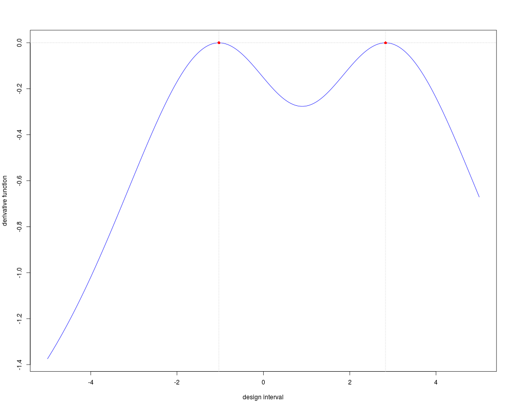
ldlogistic(a = .9 , b = .8, form = 2, lb = -5, ub = 5, user.points = c(-3, 1, 2),
           user.weights = c(.33, .33, .33))$user.eff


## Poisson model:
ymean <- yvar <-  "exp(b1 + b2 * x1)"
eff (ymean, yvar,  param = c(.9, .8), points1 = c(-3, 1, 2), points2 = c(2.5, 5.0),
     weights1 = rep(.33, 3), weights2 = c(.5, .5), prec = 54)

#####################################################################
## In the following, ymean and yvar for some famous models are given:

## Logistic model:
ymean <- "1/(exp(-b1 - b2 * x1) + 1)"
yvar <- "(1/(exp(-b1 - b2 * x1) + 1))*(1 - (1/(exp(-b1 - b2 * x1) + 1)))"

## Poisson dose response model:
ymean <- yvar <- "b1 * exp(-b2 * x1)"

## Inverse Quadratic model:
ymean <- "(b1 * x1)/(b2 + x1 + b3 * (x1)^2)"
yvar <- "1"
#
ymean <- "x1/(b1 + b2 * x1 + b3 * (x1)^2)"
yvar <- "1"

## Weibull model:
ymean <- "b1 - b2 * exp(-b3 * x1^b4)"
yvar <- "1"

## Richards model:
ymean <- "b1/(1 + b2 * exp(-b3 * x1))^b4"
yvar <- "1"

## Michaelis-Menten model:
ymean <- "(b1 * x1)/(1 + b2 * x1)"
yvar <- "1"
#
ymean <- "(b1 * x1)/(b2 + x1)"
yvar <- "1"
#
ymean <- "x1/(b1 + b2 * x1)"
yvar <- "1"

## log-linear model:
ymean <- "b1 + b2 * log(x1 + b3)"
yvar <- "1"

## Exponential model:
ymean <- "b1 + b2 * exp(x1/b3)"
yvar <- "1"

## Emax model:
ymean  <- "b1 + (b2 * x1)/(x1 + b3)"
yvar <- "1"

## Negative binomial model Y ~ NB(E(Y), theta) where E(Y) = b1 * exp(-b2 * x1):
theta <- 5
ymean <- "b1 * exp(-b2 * x1)"
yvar <- paste ("b1 * exp(-b2 * x1)*(1 + (1/", theta, ") * b1 * exp(-b2 * x1))", sep = "")

## Linear regression model:
ymean <- "b1 + b2 * x1 + b3 * x2 + b4 * x1 * x2"
yvar = "1"

Results


R version 3.3.1 (2016-06-21) -- "Bug in Your Hair"
Copyright (C) 2016 The R Foundation for Statistical Computing
Platform: x86_64-pc-linux-gnu (64-bit)

R is free software and comes with ABSOLUTELY NO WARRANTY.
You are welcome to redistribute it under certain conditions.
Type 'license()' or 'licence()' for distribution details.

R is a collaborative project with many contributors.
Type 'contributors()' for more information and
'citation()' on how to cite R or R packages in publications.

Type 'demo()' for some demos, 'help()' for on-line help, or
'help.start()' for an HTML browser interface to help.
Type 'q()' to quit R.

> library(LDOD)
Loading required package: Rsolnp
Loading required package: Rmpfr
Loading required package: gmp

Attaching package: 'gmp'

The following objects are masked from 'package:base':

    %*%, apply, crossprod, matrix, tcrossprod

C code of R package 'Rmpfr': GMP using 64 bits per limb


Attaching package: 'Rmpfr'

The following objects are masked from 'package:stats':

    dbinom, dnorm, dpois, pnorm

The following objects are masked from 'package:base':

    cbind, pmax, pmin, rbind

> png(filename="/home/ddbj/snapshot/RGM3/R_CC/result/LDOD/eff.Rd_%03d_medium.png", width=480, height=480)
> ### Name: eff
> ### Title: Calculation of D-efficiency with arbitrary precision
> ### Aliases: eff
> ### Keywords: optimal design Fisher information matrix D-efficiency
> 
> ### ** Examples
> 
> ## Logistic dose-response model
> ymean <- "(1/(exp(-b2*(x1-b1))+1))"
> yvar <- "(1/(exp(-b2*(x1-b1))+1))*(1-(1/(exp(-b2*(x1-b1))+1)))"
> eff (ymean, yvar,  param = c(.9, .8), points1 = c(-3, 1, 2), 
+      points2 = c(-1.029256,  2.829256), weights1 = rep(.33, 3), weights2 = c(.5, .5),
+      prec = 54)
1 'mpfr' number of precision  54   bits 
[1] 0.767228576575609666
> ## or
> ldlogistic(a = .9 , b = .8, form = 2, lb = -5, ub = 5, user.points = c(-3, 1, 2),
+            user.weights = c(.33, .33, .33))$user.eff

Iter: 1 fn: 2.9934	 Pars:   2.82925 -1.02926
Iter: 2 fn: 2.9934	 Pars:   2.82926 -1.02926
solnp--> Completed in 2 iterations
[1] 0.76723
> 
> 
> ## Poisson model:
> ymean <- yvar <-  "exp(b1 + b2 * x1)"
> eff (ymean, yvar,  param = c(.9, .8), points1 = c(-3, 1, 2), points2 = c(2.5, 5.0),
+      weights1 = rep(.33, 3), weights2 = c(.5, .5), prec = 54)
1 'mpfr' number of precision  54   bits 
[1] 0.0663556130781151679
> 
> #####################################################################
> ## In the following, ymean and yvar for some famous models are given:
> 
> ## Logistic model:
> ymean <- "1/(exp(-b1 - b2 * x1) + 1)"
> yvar <- "(1/(exp(-b1 - b2 * x1) + 1))*(1 - (1/(exp(-b1 - b2 * x1) + 1)))"
> 
> ## Poisson dose response model:
> ymean <- yvar <- "b1 * exp(-b2 * x1)"
> 
> ## Inverse Quadratic model:
> ymean <- "(b1 * x1)/(b2 + x1 + b3 * (x1)^2)"
> yvar <- "1"
> #
> ymean <- "x1/(b1 + b2 * x1 + b3 * (x1)^2)"
> yvar <- "1"
> 
> ## Weibull model:
> ymean <- "b1 - b2 * exp(-b3 * x1^b4)"
> yvar <- "1"
> 
> ## Richards model:
> ymean <- "b1/(1 + b2 * exp(-b3 * x1))^b4"
> yvar <- "1"
> 
> ## Michaelis-Menten model:
> ymean <- "(b1 * x1)/(1 + b2 * x1)"
> yvar <- "1"
> #
> ymean <- "(b1 * x1)/(b2 + x1)"
> yvar <- "1"
> #
> ymean <- "x1/(b1 + b2 * x1)"
> yvar <- "1"
> 
> ## log-linear model:
> ymean <- "b1 + b2 * log(x1 + b3)"
> yvar <- "1"
> 
> ## Exponential model:
> ymean <- "b1 + b2 * exp(x1/b3)"
> yvar <- "1"
> 
> ## Emax model:
> ymean  <- "b1 + (b2 * x1)/(x1 + b3)"
> yvar <- "1"
> 
> ## Negative binomial model Y ~ NB(E(Y), theta) where E(Y) = b1 * exp(-b2 * x1):
> theta <- 5
> ymean <- "b1 * exp(-b2 * x1)"
> yvar <- paste ("b1 * exp(-b2 * x1)*(1 + (1/", theta, ") * b1 * exp(-b2 * x1))", sep = "")
> 
> ## Linear regression model:
> ymean <- "b1 + b2 * x1 + b3 * x2 + b4 * x1 * x2"
> yvar = "1"
> 
> 
> 
> 
> 
> dev.off()
null device 
          1 
>