R Graphical Manual

Browse All

Last data update: 2014.03.03

R: Locally D-optimal designs for Logistic model

ldlogistic

R Documentation

Locally D-optimal designs for Logistic model

Description

Finds Locally D-optimal designs for Logistic and Logistic dose-response models which are defined as E(y) = 1/(1+exp(-a-bx)) and E(y) = 1/(1+exp(-b(x-a))) with Var(y) = E(y)(1-E(y)), respectively, where a and b are unknown parameters.

Usage

ldlogistic(a, b, form = 1 , lb, ub, user.points = NULL, user.weights = NULL, 
..., n.restarts = 1, n.sim = 1, tol = 1e-8, prec = 53, rseed = NULL)

Arguments

`a`	initial value for paremeter a.
`b`	initial value for paremeter b.
`form`	must be `1` or `2`. If `form = 1`, then E(y)=(1/(exp(-a-bx)+1)); if 'form = 2', then E(y)=1/(exp(b2(x-b1))+1).
`lb`	lower bound of design interval.
`ub`	upper bound of design interval.
`user.points`	(optional) vector of user design points which calculation of its D-efficiency is aimed. Each element of `user.points` must be within the design interval.
`user.weights`	(optional) vector of weights which its elements correspond to `user.points` elements. The sum of weights should be 1; otherwise they will be normalized.
`...`	(optional) additional parameters will be passed to function `curve`.
`prec`	(optional) a number, the maximal precision to be used for D-efficiency calculation, in bite. Must be at least 2 (default 53), see 'Details'.
`n.restarts`	(optional optimization parameter) number of solver restarts required in optimization process (default 1), see 'Details'.
`n.sim`	(optional optimization parameter) number of random parameters to generate for every restart of solver in optimization process (default 1), see 'Details'.
`tol`	(optional optimization parameter) relative tolerance on feasibility and optimality in optimization process (default 1e-8).
`rseed`	(optional optimization parameter) a seed to initiate the random number generator, else system time will be used.

Details

While D-efficiency is NaN, an increase in prec can be beneficial to achieve a numeric value, however, it can slow down the calculation speed.

Values of n.restarts and n.sim should be chosen according to the length of design interval.

Value

plot of derivative function, see 'Note'.

a list containing the following values:

`points`	obtained design points
`weights`	corresponding weights to the obtained design points
`det.value`	value of Fisher information matrix determinant at the obtained design
`user.eff`	D-efficeincy of user design, if `user.design` and `user.weights` are not `NULL`.

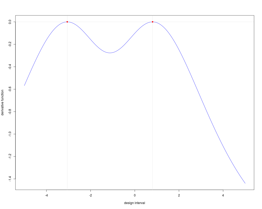
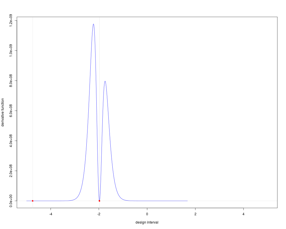
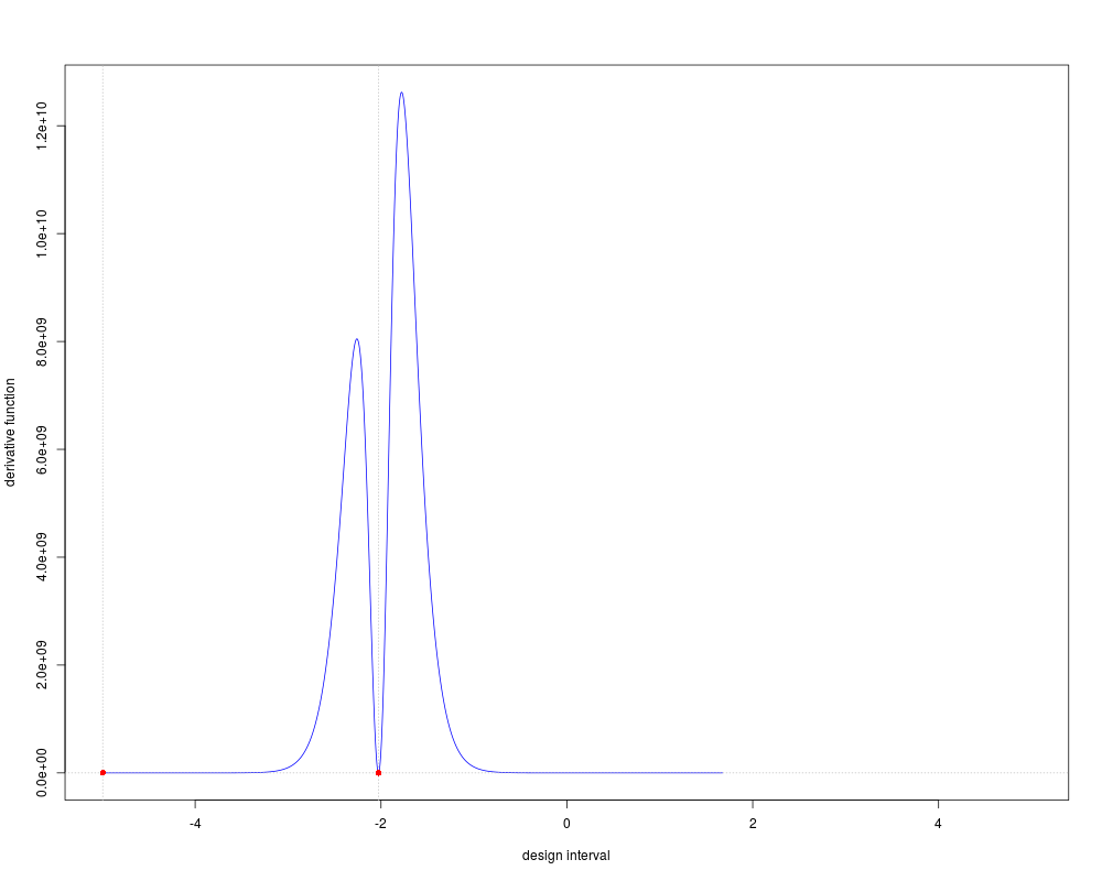
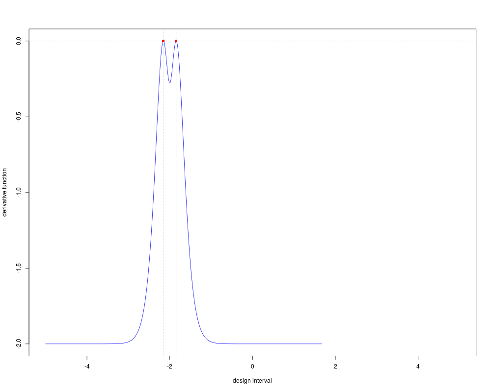
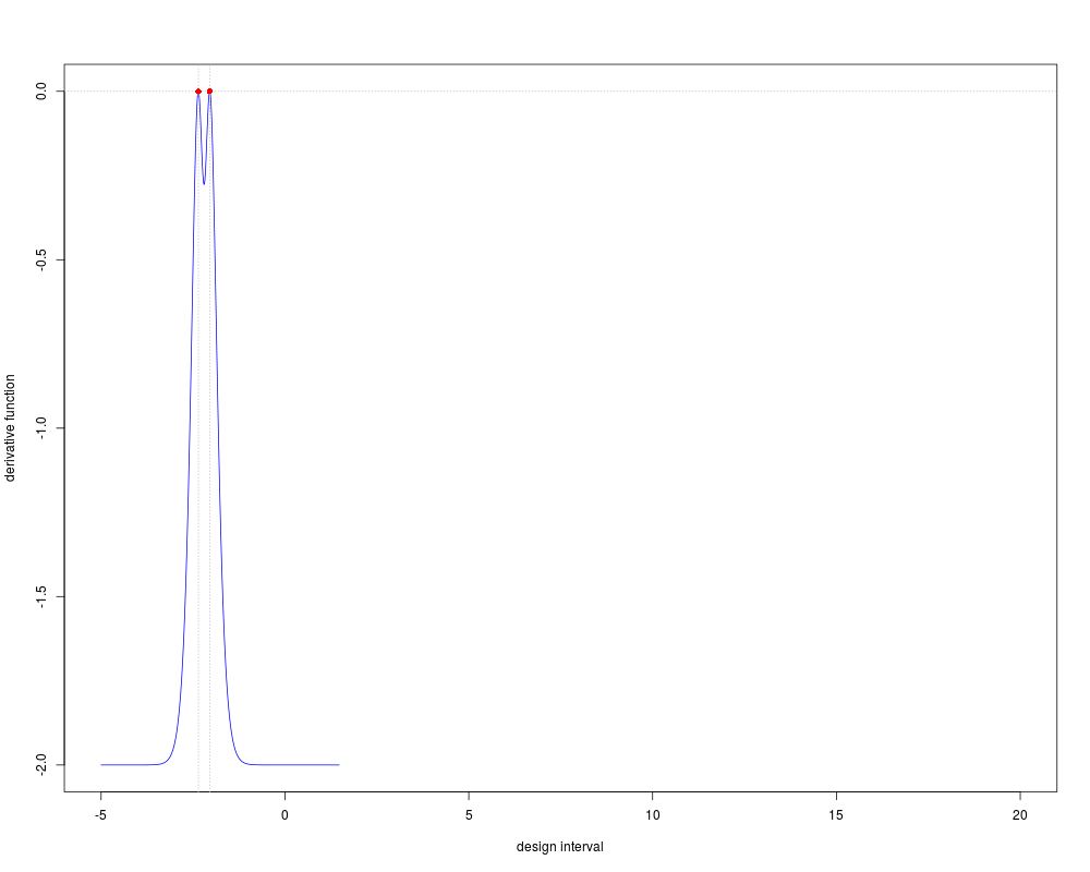
Note

To verify optimality of obtained design, derivate function (symmetry of Frechet derivative with respect to the x-axis) will be plotted on the design interval. Based on the equivalence theorem (Kiefer, 1974), a design is optimal if and only if its derivative function are equal or less than 0 on the design interval. The equality must be achieved just at the obtained points.

Author(s)

Ehsan Masoudi, Majid Sarmad and Hooshang Talebi

References

Masoudi, E., Sarmad, M. and Talebi, H. 2012, An Almost General Code in R to Find Optimal Design, In Proceedings of the 1st ISM International Statistical Conference 2012, 292-297.

Kiefer, J. C. (1974), General equivalence theory for optimum designs (approximate theory). Ann. Statist., 2, 849-879.

Examples

ldlogistic(a = .9 , b = .8, form = 1, lb = -5, ub = 5)
# $points: -3.0542559  0.8042557

## usage of n.sim and n.restars:
# Various responses for different values of rseed

ldlogistic(a = 20 , b = 10, form = 1, lb = -5, ub = 5, rseed = 9) 
# $points: -4.746680 -1.976591 

ldlogistic(a = 20 , b = 10, form = 1, lb = -5, ub = 5, rseed = 11) 
# $points -4.994817 -2.027005

ldlogistic(a = 20 , b = 10, form = 1, lb = -5, ub = 5, n.restarts = 5, n.sim = 5)
# (valid response) $points: -2.15434, -1.84566

## usage of precision:
ldlogistic(a = 22 , b = 10, form = 1, lb = -5, ub = 20, n.restarts = 7, n.sim = 7,
           user.points = c(20, 5), user.weights = c(.5, .5)) # $user.eff: NaN

ldlogistic(a = 22 , b = 10, form = 1, lb = -5, ub = 20, n.restarts = 7, n.sim = 7,
           user.points = c(20, 5), user.weights = c(.5, .5), prec = 321) # $user.eff: 0

Results


R version 3.3.1 (2016-06-21) -- "Bug in Your Hair"
Copyright (C) 2016 The R Foundation for Statistical Computing
Platform: x86_64-pc-linux-gnu (64-bit)

R is free software and comes with ABSOLUTELY NO WARRANTY.
You are welcome to redistribute it under certain conditions.
Type 'license()' or 'licence()' for distribution details.

R is a collaborative project with many contributors.
Type 'contributors()' for more information and
'citation()' on how to cite R or R packages in publications.

Type 'demo()' for some demos, 'help()' for on-line help, or
'help.start()' for an HTML browser interface to help.
Type 'q()' to quit R.

> library(LDOD)
Loading required package: Rsolnp
Loading required package: Rmpfr
Loading required package: gmp

Attaching package: 'gmp'

The following objects are masked from 'package:base':

    %*%, apply, crossprod, matrix, tcrossprod

C code of R package 'Rmpfr': GMP using 64 bits per limb


Attaching package: 'Rmpfr'

The following objects are masked from 'package:stats':

    dbinom, dnorm, dpois, pnorm

The following objects are masked from 'package:base':

    cbind, pmax, pmin, rbind

> png(filename="/home/ddbj/snapshot/RGM3/R_CC/result/LDOD/ldlogistic.Rd_%03d_medium.png", width=480, height=480)
> ### Name: ldlogistic
> ### Title: Locally D-optimal designs for Logistic model
> ### Aliases: ldlogistic
> ### Keywords: optimal design Logistic equivalence theorem
> 
> ### ** Examples
> 
> ldlogistic(a = .9 , b = .8, form = 1, lb = -5, ub = 5)

Iter: 1 fn: 2.5471	 Pars:   0.80426 -3.05426
Iter: 2 fn: 2.5471	 Pars:   0.80426 -3.05426
solnp--> Completed in 2 iterations
$points
[1] -3.0542559  0.8042557

$weights
[1] 0.5 0.5

$det.value
[1] 0.07831015

> # $points: -3.0542559  0.8042557
> 
> ## usage of n.sim and n.restars:
> # Various responses for different values of rseed
> 
> ldlogistic(a = 20 , b = 10, form = 1, lb = -5, ub = 5, rseed = 9) 

Iter: 1 fn: 28.2153	 Pars:  -1.97659 -4.74668
Iter: 2 fn: 28.2153	 Pars:  -1.97659 -4.74668
solnp--> Completed in 2 iterations
$points
[1] -4.746680 -1.976591

$weights
[1] 0.5 0.5

$det.value
[1] 5.575233e-13

> # $points: -4.746680 -1.976591 
> 
> ldlogistic(a = 20 , b = 10, form = 1, lb = -5, ub = 5, rseed = 11) 

Iter: 1 fn: 30.5632	 Pars:  -2.02701 -4.99482
Iter: 2 fn: 30.5631	 Pars:  -2.02701 -4.99482
Iter: 3 fn: 30.5631	 Pars:  -2.02701 -4.99482
solnp--> Completed in 3 iterations
$points
[1] -4.994817 -2.027005

$weights
[1] 0.5 0.5

$det.value
[1] 5.328602e-14

> # $points -4.994817 -2.027005
> 
> ldlogistic(a = 20 , b = 10, form = 1, lb = -5, ub = 5, n.restarts = 5, n.sim = 5)

Iter: 1 fn: 7.5985	 Pars:  -2.15434 -1.84566
Iter: 2 fn: 7.5985	 Pars:  -2.15434 -1.84566
solnp--> Completed in 2 iterations

Iter: 1 fn: 7.5985	 Pars:  -2.15434 -1.84566
Iter: 2 fn: 7.5985	 Pars:  -2.15434 -1.84566
solnp--> Completed in 2 iterations

Iter: 1 fn: 26.6366	 Pars:  -1.98475 -4.57627
Iter: 2 fn: 26.6366	 Pars:  -1.98475 -4.57627
solnp--> Completed in 2 iterations

Iter: 1 fn: 7.5985	 Pars:  -2.15434 -1.84566
Iter: 2 fn: 7.5985	 Pars:  -2.15434 -1.84566
solnp--> Completed in 2 iterations

Iter: 1 fn: 7.5985	 Pars:  -2.15434 -1.84566
Iter: 2 fn: 7.5985	 Pars:  -2.15434 -1.84566
solnp--> Completed in 2 iterations
$points
[1] -2.15434 -1.84566

$weights
[1] 0.5 0.5

$det.value
[1] 0.0005011849

> # (valid response) $points: -2.15434, -1.84566
> 
> ## usage of precision:
> ldlogistic(a = 22 , b = 10, form = 1, lb = -5, ub = 20, n.restarts = 7, n.sim = 7,
+            user.points = c(20, 5), user.weights = c(.5, .5)) # $user.eff: NaN

Iter: 1 fn: 25.8033	 Pars:  -4.67603 -2.24394
Iter: 2 fn: 25.8033	 Pars:  -4.67603 -2.24394
solnp--> Completed in 2 iterations

Iter: 1 fn: 28.0054	 Pars:   0.51645 -2.26917
Iter: 2 fn: 28.0054	 Pars:   0.51645 -2.26917
solnp--> Completed in 2 iterations

Iter: 1 fn: 1e+24	 Pars:  14.46455  6.20211
Iter: 1 fn: 1e+24	 Pars:   8.11300 15.60595
Iter: 1 fn: 1e+24	 Pars:  11.68293 -1.05647
Iter: 1 fn: 1e+24	 Pars:  11.32653  3.56996
Iter: 1 fn: 1e+24	 Pars:  14.85849  6.42258$points
[1] -4.676032 -2.243944

$weights
[1] 0.5 0.5

$det.value
[1] 6.219745e-12

$user.eff
[1] NaN

> 
> ldlogistic(a = 22 , b = 10, form = 1, lb = -5, ub = 20, n.restarts = 7, n.sim = 7,
+            user.points = c(20, 5), user.weights = c(.5, .5), prec = 321) # $user.eff: 0

Iter: 1 fn: 7.5985	 Pars:  -2.04566 -2.35434
Iter: 2 fn: 7.5985	 Pars:  -2.04566 -2.35434
solnp--> Completed in 2 iterations

Iter: 1 fn: 7.5985	 Pars:  -2.04566 -2.35434
Iter: 2 fn: 7.5985	 Pars:  -2.04566 -2.35434
solnp--> Completed in 2 iterations

Iter: 1 fn: 7.5985	 Pars:  -2.35434 -2.04566
Iter: 2 fn: 7.5985	 Pars:  -2.35434 -2.04566
solnp--> Completed in 2 iterations

Iter: 1 fn: 7.5985	 Pars:  -2.35434 -2.04566
Iter: 2 fn: 7.5985	 Pars:  -2.35434 -2.04566
solnp--> Completed in 2 iterations

Iter: 1 fn: 1e+24	 Pars:  19.09814  6.58379
Iter: 1 fn: 1e+24	 Pars:  -4.30973 13.21338
Iter: 1 fn: 1e+24	 Pars:  11.63128 -2.47791$points
[1] -2.354341 -2.045660

$weights
[1] 0.5 0.5

$det.value
[1] 0.0005011849

$user.eff
[1] 0

> 
> 
> 
> 
> 
> dev.off()
null device 
          1 
>