Function to Average Orthogonal Projection Matrices

Description

The function computes the average of orthogonal projection matrices and estimates the average rank.

Usage

AOP(x, weights = "constant")

Arguments

Details

The AOP maximizes the function D(P)= w(k)tr(P.bar_w P)- 0.5w^2(k)k, where P.bar_w=1/m sum(w(k_i) P_i) is a regular average of weighted orthogonal projection matrices, m is the number of orthogonal projection matrices averaged, w(k)is the weight function and k is the rank of P. The possible weights are defined as constant: w(k)=1, inverse: w(k)=1/k and sq.inverse: w(k)=1/sqrt(k). The constant weight corresponds to the so called Crone & Crosby distance. Orthogonal projection matrices of zero rank are also possible inputs for the function. In such a case, the function prints a warning giving the number of orthogonal projection matrices with zero rank.

Value

A list containing the following components:

Author(s)

Eero Liski and Klaus Nordhausen

References

Crone, L. J., and Crosby, D. S. (1995), Statistical Applications of a Metric on Subspaces to Satellite Meteorology, Technometrics 37, 324-328.

Liski, E., Nordhausen, K., Oja, H. and Ruiz-Gazen, A. (201?), Combining Linear Dimension Reduction Subspaces, to appear in the proceedings of ICORS 2015.

See Also

Pdist

Examples

## Ex.1
##
library(dr)
# Australian athletes data with 202 observations
data(ais)
# 10 explanatory variables
X <- as.matrix(ais[,c(2:3,5:12)])
colnames(X) <- names(ais[,c(2:3,5:12)])
p <- dim(X)[2]
# Response variable lean body mass (LBM)
y <- ais$LBM
# Significance level 
alpha <- 0.05


# SIR
s0.sir <- dr(y ~ X, method="sir")
# Estimate of k 
k.sir <- sum(dr.test(s0.sir, numdir=4)[,3] < alpha)
# List of transformation matrices corresponding to 
# k.sir and fixed k=1, respectively
B.sir.list <- list(B1=s0.sir$evectors[,1:k.sir], B2=s0.sir$evectors[,1:1])
# List of orthogonal projectors corresponding to 
# k.sir, fixed k=1 and fixed k=0, respectively
P.sir.list <- list(P1=O2P(B.sir.list$B1), P2=O2P(B.sir.list$B2), 
P3=diag(0,p))


# SAVE
s0.save <- dr(y ~ X, method="save")
# Estimate of k 
k.save <- sum(dr.test(s0.save, numdir=4)[,3] < alpha)
# List of transformation matrices corresponding to 
# k.save and fixed k=1, respectively
B.save.list <- list(B1=s0.save$evectors[,1:k.save], 
B2=s0.save$evectors[,1:1])
# List of orthogonal projectors corresponding to 
# k.save, fixed k=1 and fixed k=0, respectively
P.save.list <- list(P1=O2P(B.save.list$B1), P2=O2P(B.save.list$B2), 
P3=diag(0,p))


# DR k-estimates
dr.k <- c(k.sir, k.save)
names(dr.k) <- c("SIR","SAVE")
dr.k


# List of individually estimated projectors
proj.list.a <- list(P.sir.list$P1, P.save.list$P1)
# List of fixed projectors
proj.list.b <- list(P.sir.list$P2, P.save.list$P2)
# List of zero projectors
proj.list.c <- list(P.sir.list$P3, P.save.list$P3)
# List of zero-rank SIR-projector and 
# other individually estimated projectors
proj.list.d <- list(P.sir.list$P3, P.save.list$P1)


# AOP (constant) object corresponding to the first projector list
AOP.const.a <- AOP(proj.list.a, weights="constant")

# AOP (inverse) objects corresponding to three projector lists
AOP.inv.a <- AOP(proj.list.a, weights="inverse")
AOP.inv.b <- AOP(proj.list.b, weights="inverse")
AOP.inv.c <- AOP(proj.list.c, weights="inverse")

# AOP (sq.inverse) objects corresponding to three projector lists
AOP.sqinv.a <- AOP(proj.list.a, weights="sq.inverse")
AOP.sqinv.c <- AOP(proj.list.c, weights="sq.inverse")
AOP.sqinv.d <- AOP(proj.list.d, weights="sq.inverse")


# k-estimates of the AOP's
AOP.a <- c(AOP.const.a$k, AOP.inv.a$k, AOP.sqinv.a$k)
names(AOP.a) <- c("const","inv","sqinv")
AOP.a

AOP.c <- AOP.inv.c$k
names(AOP.c) <- c("inv")
AOP.c

AOP.d <- AOP.sqinv.d$k
names(AOP.d) <- c("sqinv")
AOP.d


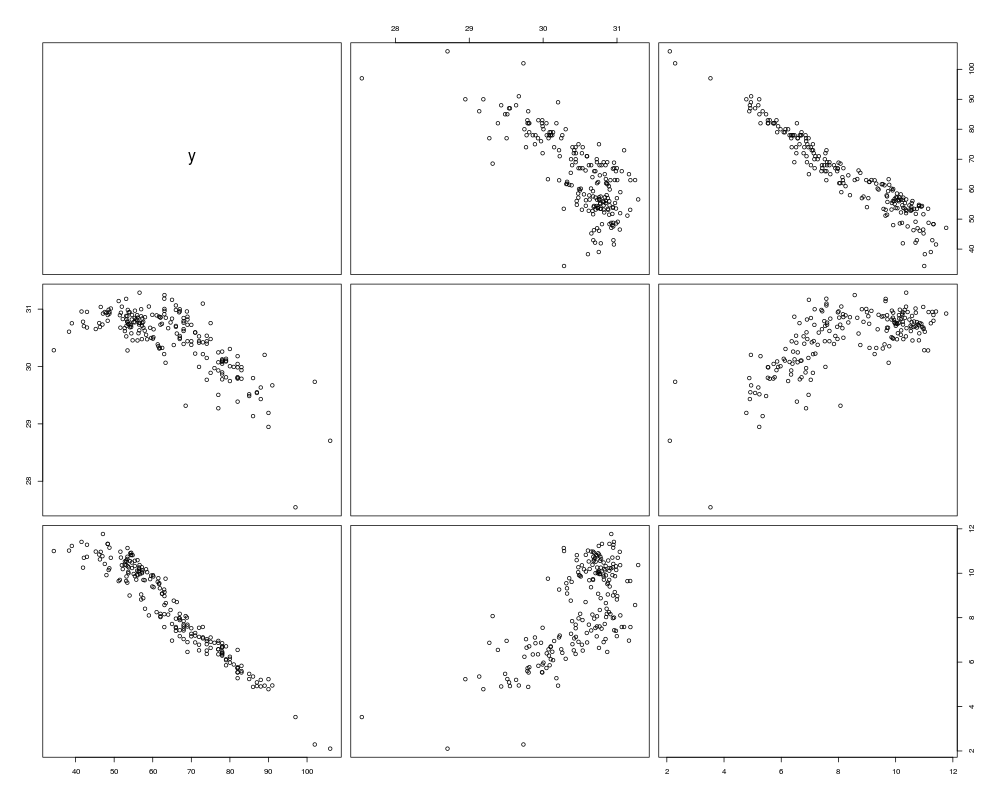
# Scatter plots between the response and the transformed data 
# corresponding to the different AOP transformation matrices

# AOP.inverse
newdata.inv.AOPa <- cbind(y,X %*% AOP.inv.a$O)
pairs(newdata.inv.AOPa)

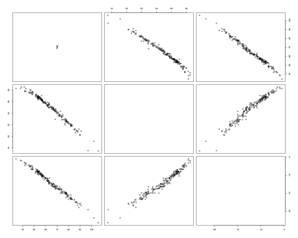
newdata.inv.AOPb <- cbind(y,X %*% AOP.inv.b$O)
pairs(newdata.inv.AOPb)


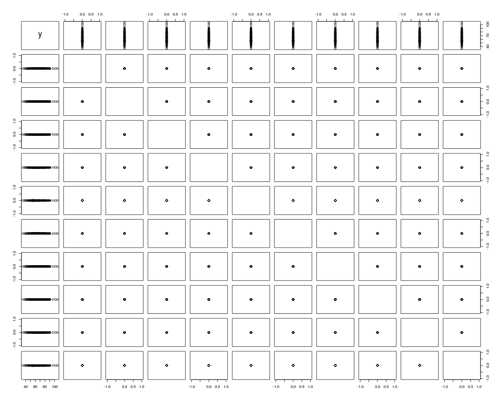
# AOP.sq.inverse
newdata.sqinv.AOPc <- cbind(y,X %*% AOP.sqinv.c$O)
pairs(newdata.sqinv.AOPc)

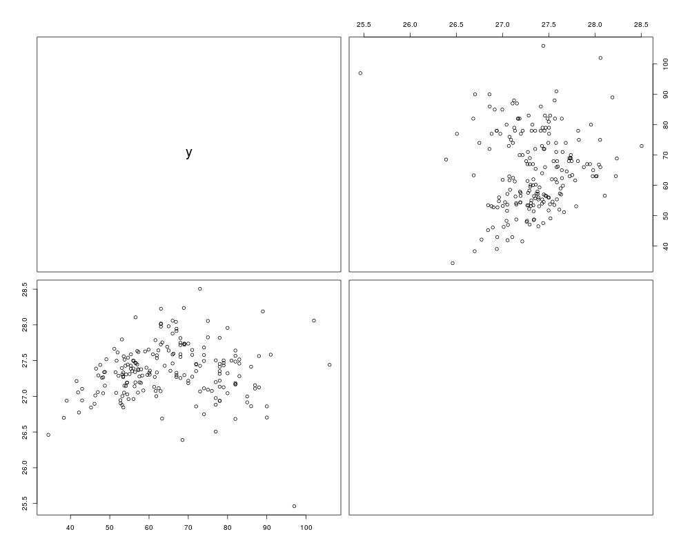
newdata.sqinv.AOPd <- cbind(y,X %*% AOP.sqinv.d$O)
pairs(newdata.sqinv.AOPd)






###################################
## Ex.2
##
a <- c(1,1,rep(0,8))
A <- diag(a)
B <- diag(0,10)
B[3,1] <- 1
P.A <- O2P(A[,1:2])
P.B <- O2P(B[,1])
zero.mat <- diag(0,10)
# True projector, k=3
P.C <- P.A + P.B

# Average P.A and P.B
proj.list <- list(P.A, P.B)
AOP.const <- AOP(proj.list, weights="constant")
AOP.inv <- AOP(proj.list, weights="inverse")
AOP.sqinv <- AOP(proj.list, weights="sq.inverse")
k.list <- c(AOP.const$k, AOP.inv$k, AOP.sqinv$k)
names(k.list) <- c("const","inv","sqinv")
k.list

# Average P.A, P.B and three zero rank matrices
proj.list <- list(P.A, P.B, zero.mat, zero.mat, zero.mat)
AOP.const <- AOP(proj.list, weights="constant")
AOP.inv <- AOP(proj.list, weights="inverse")
AOP.sqinv <- AOP(proj.list, weights="sq.inverse")
k.list <- c(AOP.const$k, AOP.inv$k, AOP.sqinv$k)
names(k.list) <- c("const","inv","sqinv")
k.list

Results

R version 3.3.1 (2016-06-21) -- "Bug in Your Hair"
Copyright (C) 2016 The R Foundation for Statistical Computing
Platform: x86_64-pc-linux-gnu (64-bit)

R is free software and comes with ABSOLUTELY NO WARRANTY.
You are welcome to redistribute it under certain conditions.
Type 'license()' or 'licence()' for distribution details.

R is a collaborative project with many contributors.
Type 'contributors()' for more information and
'citation()' on how to cite R or R packages in publications.

Type 'demo()' for some demos, 'help()' for on-line help, or
'help.start()' for an HTML browser interface to help.
Type 'q()' to quit R.

> library(LDRTools)
> png(filename="/home/ddbj/snapshot/RGM3/R_CC/result/LDRTools/AOP.Rd_%03d_medium.png", width=480, height=480)
> ### Name: AOP
> ### Title: Function to Average Orthogonal Projection Matrices
> ### Aliases: AOP
> ### Keywords: multivariate
> 
> ### ** Examples
> 
> ## Ex.1
> ##
> library(dr)
Loading required package: MASS
> # Australian athletes data with 202 observations
> data(ais)
> # 10 explanatory variables
> X <- as.matrix(ais[,c(2:3,5:12)])
> colnames(X) <- names(ais[,c(2:3,5:12)])
> p <- dim(X)[2]
> # Response variable lean body mass (LBM)
> y <- ais$LBM
> # Significance level 
> alpha <- 0.05
> 
> 
> # SIR
> s0.sir <- dr(y ~ X, method="sir")
> # Estimate of k 
> k.sir <- sum(dr.test(s0.sir, numdir=4)[,3] < alpha)
> # List of transformation matrices corresponding to 
> # k.sir and fixed k=1, respectively
> B.sir.list <- list(B1=s0.sir$evectors[,1:k.sir], B2=s0.sir$evectors[,1:1])
> # List of orthogonal projectors corresponding to 
> # k.sir, fixed k=1 and fixed k=0, respectively
> P.sir.list <- list(P1=O2P(B.sir.list$B1), P2=O2P(B.sir.list$B2), 
+ P3=diag(0,p))
> 
> 
> # SAVE
> s0.save <- dr(y ~ X, method="save")
> # Estimate of k 
> k.save <- sum(dr.test(s0.save, numdir=4)[,3] < alpha)
> # List of transformation matrices corresponding to 
> # k.save and fixed k=1, respectively
> B.save.list <- list(B1=s0.save$evectors[,1:k.save], 
+ B2=s0.save$evectors[,1:1])
> # List of orthogonal projectors corresponding to 
> # k.save, fixed k=1 and fixed k=0, respectively
> P.save.list <- list(P1=O2P(B.save.list$B1), P2=O2P(B.save.list$B2), 
+ P3=diag(0,p))
> 
> 
> # DR k-estimates
> dr.k <- c(k.sir, k.save)
> names(dr.k) <- c("SIR","SAVE")
> dr.k
 SIR SAVE 
   3    1 
> 
> 
> # List of individually estimated projectors
> proj.list.a <- list(P.sir.list$P1, P.save.list$P1)
> # List of fixed projectors
> proj.list.b <- list(P.sir.list$P2, P.save.list$P2)
> # List of zero projectors
> proj.list.c <- list(P.sir.list$P3, P.save.list$P3)
> # List of zero-rank SIR-projector and 
> # other individually estimated projectors
> proj.list.d <- list(P.sir.list$P3, P.save.list$P1)
> 
> 
> # AOP (constant) object corresponding to the first projector list
> AOP.const.a <- AOP(proj.list.a, weights="constant")
> 
> # AOP (inverse) objects corresponding to three projector lists
> AOP.inv.a <- AOP(proj.list.a, weights="inverse")
> AOP.inv.b <- AOP(proj.list.b, weights="inverse")
> AOP.inv.c <- AOP(proj.list.c, weights="inverse")
Warning message:
In AOP.inverse(x) : There are  2  projectors with rank 0
> 
> # AOP (sq.inverse) objects corresponding to three projector lists
> AOP.sqinv.a <- AOP(proj.list.a, weights="sq.inverse")
> AOP.sqinv.c <- AOP(proj.list.c, weights="sq.inverse")
Warning message:
In AOP.sq.inverse(x) : There are  2  projectors with rank 0
> AOP.sqinv.d <- AOP(proj.list.d, weights="sq.inverse")
Warning message:
In AOP.sq.inverse(x) : There are  1  projectors with rank 0
> 
> 
> # k-estimates of the AOP's
> AOP.a <- c(AOP.const.a$k, AOP.inv.a$k, AOP.sqinv.a$k)
> names(AOP.a) <- c("const","inv","sqinv")
> AOP.a
const   inv sqinv 
    2     2     2 
> 
> AOP.c <- AOP.inv.c$k
> names(AOP.c) <- c("inv")
> AOP.c
inv 
  0 
> 
> AOP.d <- AOP.sqinv.d$k
> names(AOP.d) <- c("sqinv")
> AOP.d
sqinv 
    1 
> 
> 
> # Scatter plots between the response and the transformed data 
> # corresponding to the different AOP transformation matrices
> 
> # AOP.inverse
> newdata.inv.AOPa <- cbind(y,X %*% AOP.inv.a$O)
> pairs(newdata.inv.AOPa)
> 
> newdata.inv.AOPb <- cbind(y,X %*% AOP.inv.b$O)
> pairs(newdata.inv.AOPb)
> 
> 
> # AOP.sq.inverse
> newdata.sqinv.AOPc <- cbind(y,X %*% AOP.sqinv.c$O)
> pairs(newdata.sqinv.AOPc)
> 
> newdata.sqinv.AOPd <- cbind(y,X %*% AOP.sqinv.d$O)
> pairs(newdata.sqinv.AOPd)
> 
> 
> 
> 
> 
> 
> ###################################
> ## Ex.2
> ##
> a <- c(1,1,rep(0,8))
> A <- diag(a)
> B <- diag(0,10)
> B[3,1] <- 1
> P.A <- O2P(A[,1:2])
> P.B <- O2P(B[,1])
> zero.mat <- diag(0,10)
> # True projector, k=3
> P.C <- P.A + P.B
> 
> # Average P.A and P.B
> proj.list <- list(P.A, P.B)
> AOP.const <- AOP(proj.list, weights="constant")
> AOP.inv <- AOP(proj.list, weights="inverse")
> AOP.sqinv <- AOP(proj.list, weights="sq.inverse")
> k.list <- c(AOP.const$k, AOP.inv$k, AOP.sqinv$k)
> names(k.list) <- c("const","inv","sqinv")
> k.list
const   inv sqinv 
    3     3     3 
> 
> # Average P.A, P.B and three zero rank matrices
> proj.list <- list(P.A, P.B, zero.mat, zero.mat, zero.mat)
> AOP.const <- AOP(proj.list, weights="constant")
Warning message:
In AOP.constant(x) : There are  3  projectors with rank 0
> AOP.inv <- AOP(proj.list, weights="inverse")
Warning message:
In AOP.inverse(x) : There are  3  projectors with rank 0
> AOP.sqinv <- AOP(proj.list, weights="sq.inverse")
Warning message:
In AOP.sq.inverse(x) : There are  3  projectors with rank 0
> k.list <- c(AOP.const$k, AOP.inv$k, AOP.sqinv$k)
> names(k.list) <- c("const","inv","sqinv")
> k.list
const   inv sqinv 
    3     3     3 
> 
> 
> 
> 
> 
> 
> dev.off()
null device 
          1 
>