Supported by Dr. Osamu Ogasawara and  . . |
|
Last data update: 2014.03.03 |
This function produces a pairwise LD plot.Description
UsageLDheatmap(gdat, genetic.distances=NULL, distances="physical", LDmeasure="r", title="Pairwise LD", add.map=TRUE, add.key=TRUE, geneMapLocation=0.15, geneMapLabelX=NULL, geneMapLabelY=NULL, SNP.name=NULL, color=NULL, newpage=TRUE, name="ldheatmap", vp.name=NULL, pop=FALSE, flip=NULL, text=FALSE) Arguments
DetailsFor For the argument See the package vignette ValueAn object of class
The
Note The produced heat map can be modified in two ways.
First, it is possible to edit interactively the grob components of the heat map,
by using the function
Author(s)Ji-hyung Shin <shin@sfu.ca>, Sigal Blay <sblay@sfu.ca>, Nicholas Lewin-Koh <nikko@hailmail.net>, Brad McNeney <mcneney@stat.sfu.ca>, Jinko Graham <jgraham@cs.sfu.ca> ReferencesShin J-H, Blay S, McNeney B and Graham J (2006). LDheatmap: An R Function for Graphical Display of Pairwise Linkage Disequilibria Between Single Nucleotide Polymorphisms. Journal of Statistical Software, 16 Code Snippet 3 See Also
Examples
#Load the package's data set
data(CEUData)
#Creates a data frame "CEUSNP" of genotype data and a vector "CEUDist"
#of physical locations of the SNPs
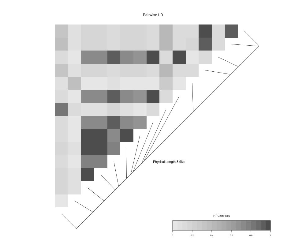
# Produce a heat map in a grey color scheme
MyHeatmap <- LDheatmap(CEUSNP, genetic.distances = CEUDist,
color = grey.colors(20))
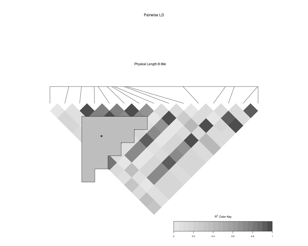
# Same heatmap, flipped below a horizontal gene map -- for examples of
# adding genomic annotation tracks to a flipped heatmap see
# vignette("addTracks")
flippedHeatmap<-LDheatmap(MyHeatmap,flip=TRUE)
# Prompt the user before starting a new page of graphics output
# and save the original prompt settings in old.prompt.
old.prompt <- devAskNewPage(ask = TRUE)
# Highlight a certain LD block of interest:
LDheatmap.highlight(MyHeatmap, i = 3, j = 8, col = "black", fill = "grey" )
# Plot a symbol in the center of the pixel which represents LD between
# the fourth and seventh SNPs:
LDheatmap.marks(MyHeatmap, 4, 7, gp=gpar(cex=2), pch = "*")
#### Use an RGB pallete for the color scheme ####
rgb.palette <- colorRampPalette(rev(c("blue", "orange", "red")), space = "rgb")
LDheatmap(MyHeatmap, color=rgb.palette(18))
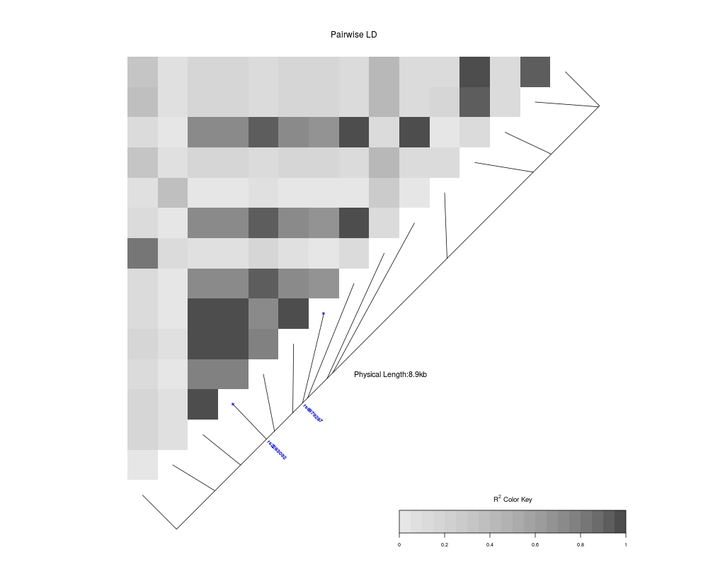
#### Modify the plot by using 'grid.edit' function ####
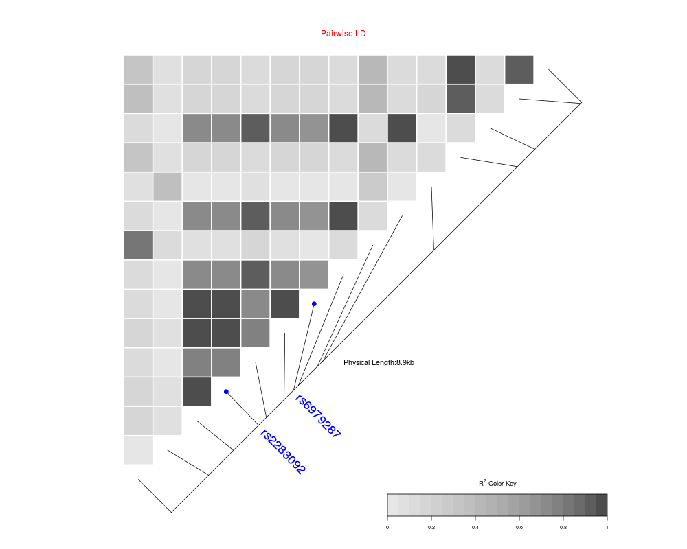
#Draw a heat map where the SNPs "rs2283092" and "rs6979287" are labelled.
LDheatmap(MyHeatmap, SNP.name = c("rs2283092", "rs6979287"))
#Find the names of the top-level graphical objects (grobs) on the current display
getNames()
#[1] "ldheatmap"
# Find the names of the component grobs of "ldheatmap"
childNames(grid.get("ldheatmap"))
#[1] "heatMap" "geneMap" "Key"
#Find the names of the component grobs of heatMap
childNames(grid.get("heatMap"))
#[1] "heatmap" "title"
#Find the names of the component grobs of geneMap
childNames(grid.get("geneMap"))
#[1] "diagonal" "segments" "title" "symbols" "SNPnames"
#Find the names of the component grobs of Key
childNames(grid.get("Key"))
#[1] "colorKey" "title" "labels" "ticks" "box"
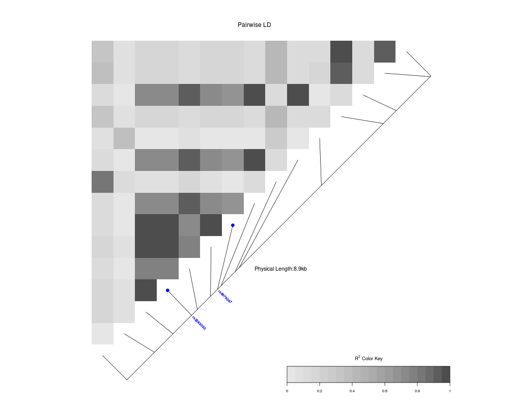
#Change the plotting symbols that identify SNPs rs2283092 and rs6979287
#on the plot to bullets
grid.edit("symbols", pch = 20, gp = gpar(cex = 1))
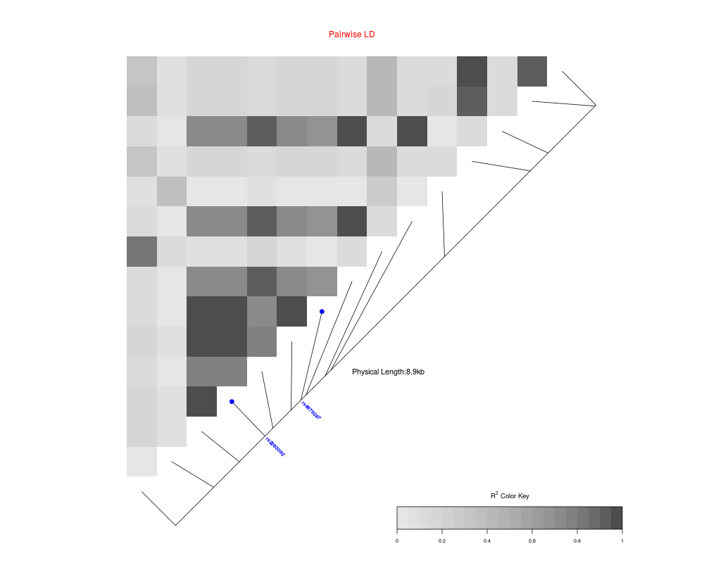
#Change the color of the main title
grid.edit(gPath("ldheatmap", "heatMap", "title"), gp = gpar(col = "red"))
#Change size of SNP labels
grid.edit(gPath("ldheatmap", "geneMap","SNPnames"), gp = gpar(cex=1.5))
#Add a grid of white lines to the plot to separate pairwise LD measures
grid.edit(gPath("ldheatmap", "heatMap", "heatmap"), gp = gpar(col = "white",
lwd = 2))
#### Modify a heat map using 'editGrob' function ####
MyHeatmap <- LDheatmap(MyHeatmap, color = grey.colors(20))
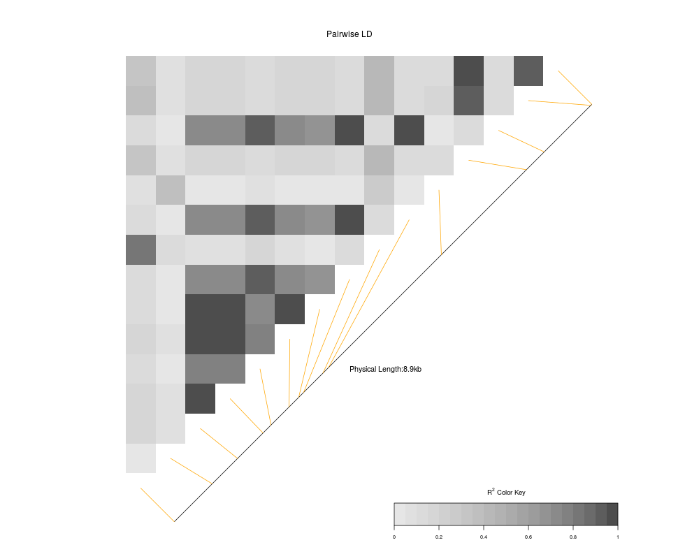
new.grob <- editGrob(MyHeatmap$LDheatmapGrob, gPath("geneMap", "segments"),
gp=gpar(col="orange"))
##Clear the old graphics object from the display before drawing the modified heat map:
grid.newpage()
grid.draw(new.grob)
# now the colour of line segments connecting the SNP
# positions to the LD heat map has been changed from black to orange.
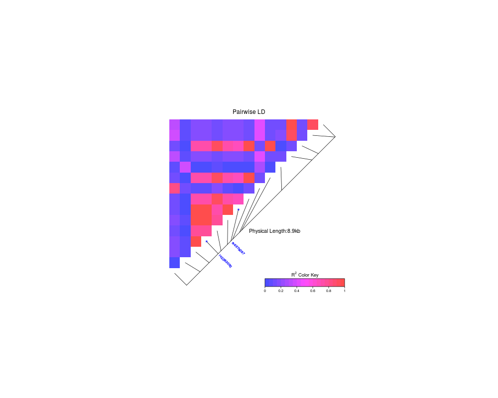
#### Draw a resized heat map (in a 'blue-to-red' color scale ####
grid.newpage()
pushViewport(viewport(width=0.5, height=0.5))
LDheatmap(MyHeatmap, SNP.name = c("rs2283092", "rs6979287"), newpage=FALSE,
color="blueToRed")
popViewport()
#### Draw and modify two heat maps on one plot ####
grid.newpage()
##Draw and the first heat map on the left half of the graphics device
pushViewport(viewport(x=0, width=0.5, just="left"))
LD1<-LDheatmap(MyHeatmap, color=grey.colors(20), newpage=FALSE,
title="Pairwise LD in grey.colors(20)",
SNP.name="rs6979572", geneMapLabelX=0.6,
geneMapLabelY=0.4, name="ld1")
upViewport()
##Draw the second heat map on the right half of the graphics device
pushViewport(viewport(x=1,width=0.5,just="right"))
LD2<-LDheatmap(MyHeatmap, newpage=FALSE, title="Pairwise LD in heat.colors(20)",
SNP.name="rs6979572", geneMapLabelX=0.6, geneMapLabelY=0.4, name="ld2")
upViewport()
##Modify the text size of main title of the first heat map.
grid.edit(gPath("ld1", "heatMap","title"), gp=gpar(cex=1.5))
##Modify the text size and color of the SNP label of the second heat map.
grid.edit(gPath("ld2", "geneMap","SNPnames"), gp=gpar(cex=1.5, col="DarkRed"))
#### Draw a lattice-like plot with heat maps in panels ####
# Load CHBJPTSNP and CHBJPTDist
data(CHBJPTData)
# Make a variable which indicates Chinese vs. Japanese
pop <- factor(c(rep("chinese",45), rep("japanese",45)))
require(lattice)
xyplot(1:nrow(CHBJPTSNP) ~ 1:nrow(CHBJPTSNP) | pop,
type="n", scales=list(draw=FALSE), xlab="", ylab="",
panel=function(x, y, subscripts,...) {
LDheatmap(CHBJPTSNP[subscripts,], CHBJPTDist, newpage=FALSE) })
data(GIMAP5)
require(lattice)
n<-nrow(GIMAP5$snp.data)
xyplot(1:n ~ 1:n | GIMAP5$subject.support$pop,
type="n", scales=list(draw=FALSE), xlab="", ylab="",
panel=function(x, y, subscripts,...) {
LDheatmap(GIMAP5$snp.data[subscripts,],
GIMAP5$snp.support$Position, SNP.name="rs6598", newpage=FALSE) })
#Reset the user's setting for prompting on the graphics output
#to the original value before running these example commands.
devAskNewPage(old.prompt)
Results
R version 3.3.1 (2016-06-21) -- "Bug in Your Hair"
Copyright (C) 2016 The R Foundation for Statistical Computing
Platform: x86_64-pc-linux-gnu (64-bit)
R is free software and comes with ABSOLUTELY NO WARRANTY.
You are welcome to redistribute it under certain conditions.
Type 'license()' or 'licence()' for distribution details.
R is a collaborative project with many contributors.
Type 'contributors()' for more information and
'citation()' on how to cite R or R packages in publications.
Type 'demo()' for some demos, 'help()' for on-line help, or
'help.start()' for an HTML browser interface to help.
Type 'q()' to quit R.
> library(LDheatmap)
Loading required package: grid
> png(filename="/home/ddbj/snapshot/RGM3/R_CC/result/LDheatmap/LDheatmap.Rd_%03d_medium.png", width=480, height=480)
> ### Name: LDheatmap
> ### Title: This function produces a pairwise LD plot.
> ### Aliases: LDheatmap
> ### Keywords: hplot
>
> ### ** Examples
>
> #Load the package's data set
> data(CEUData)
> #Creates a data frame "CEUSNP" of genotype data and a vector "CEUDist"
> #of physical locations of the SNPs
>
> # Produce a heat map in a grey color scheme
>
> MyHeatmap <- LDheatmap(CEUSNP, genetic.distances = CEUDist,
+ color = grey.colors(20))
>
> # Same heatmap, flipped below a horizontal gene map -- for examples of
> # adding genomic annotation tracks to a flipped heatmap see
> # vignette("addTracks")
>
> flippedHeatmap<-LDheatmap(MyHeatmap,flip=TRUE)
>
> # Prompt the user before starting a new page of graphics output
> # and save the original prompt settings in old.prompt.
> old.prompt <- devAskNewPage(ask = TRUE)
>
> # Highlight a certain LD block of interest:
> LDheatmap.highlight(MyHeatmap, i = 3, j = 8, col = "black", fill = "grey" )
> # Plot a symbol in the center of the pixel which represents LD between
> # the fourth and seventh SNPs:
> LDheatmap.marks(MyHeatmap, 4, 7, gp=gpar(cex=2), pch = "*")
>
>
> #### Use an RGB pallete for the color scheme ####
> rgb.palette <- colorRampPalette(rev(c("blue", "orange", "red")), space = "rgb")
> LDheatmap(MyHeatmap, color=rgb.palette(18))
>
>
> #### Modify the plot by using 'grid.edit' function ####
> #Draw a heat map where the SNPs "rs2283092" and "rs6979287" are labelled.
> LDheatmap(MyHeatmap, SNP.name = c("rs2283092", "rs6979287"))
>
> #Find the names of the top-level graphical objects (grobs) on the current display
> getNames()
[1] "ldheatmap"
> #[1] "ldheatmap"
>
> # Find the names of the component grobs of "ldheatmap"
> childNames(grid.get("ldheatmap"))
[1] "heatMap" "geneMap" "Key"
> #[1] "heatMap" "geneMap" "Key"
>
> #Find the names of the component grobs of heatMap
> childNames(grid.get("heatMap"))
[1] "heatmap" "title"
> #[1] "heatmap" "title"
>
> #Find the names of the component grobs of geneMap
> childNames(grid.get("geneMap"))
[1] "diagonal" "segments" "title" "symbols" "SNPnames"
> #[1] "diagonal" "segments" "title" "symbols" "SNPnames"
>
> #Find the names of the component grobs of Key
> childNames(grid.get("Key"))
[1] "colorKey" "title" "labels" "ticks" "box"
> #[1] "colorKey" "title" "labels" "ticks" "box"
>
> #Change the plotting symbols that identify SNPs rs2283092 and rs6979287
> #on the plot to bullets
> grid.edit("symbols", pch = 20, gp = gpar(cex = 1))
>
> #Change the color of the main title
> grid.edit(gPath("ldheatmap", "heatMap", "title"), gp = gpar(col = "red"))
>
> #Change size of SNP labels
> grid.edit(gPath("ldheatmap", "geneMap","SNPnames"), gp = gpar(cex=1.5))
>
> #Add a grid of white lines to the plot to separate pairwise LD measures
> grid.edit(gPath("ldheatmap", "heatMap", "heatmap"), gp = gpar(col = "white",
+ lwd = 2))
>
>
> #### Modify a heat map using 'editGrob' function ####
> MyHeatmap <- LDheatmap(MyHeatmap, color = grey.colors(20))
>
> new.grob <- editGrob(MyHeatmap$LDheatmapGrob, gPath("geneMap", "segments"),
+ gp=gpar(col="orange"))
>
> ##Clear the old graphics object from the display before drawing the modified heat map:
> grid.newpage()
>
> grid.draw(new.grob)
> # now the colour of line segments connecting the SNP
> # positions to the LD heat map has been changed from black to orange.
>
>
> #### Draw a resized heat map (in a 'blue-to-red' color scale ####
> grid.newpage()
>
> pushViewport(viewport(width=0.5, height=0.5))
> LDheatmap(MyHeatmap, SNP.name = c("rs2283092", "rs6979287"), newpage=FALSE,
+ color="blueToRed")
> popViewport()
>
>
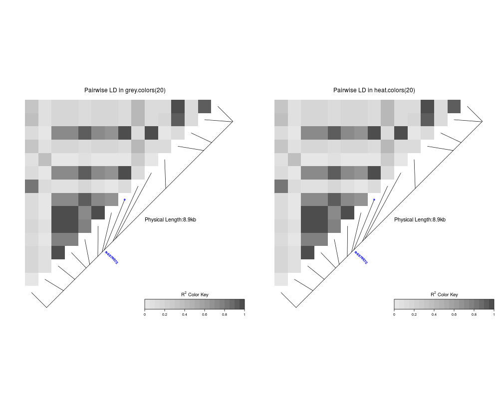
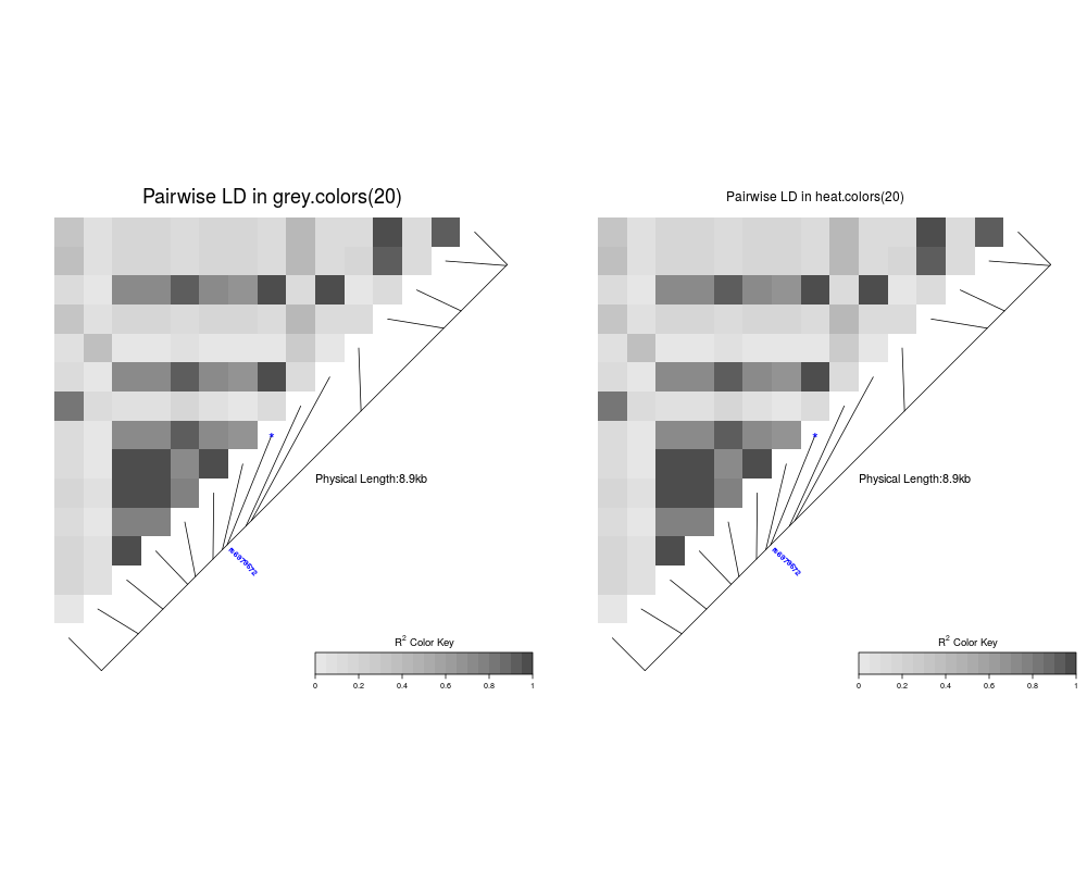
> #### Draw and modify two heat maps on one plot ####
> grid.newpage()
>
> ##Draw and the first heat map on the left half of the graphics device
> pushViewport(viewport(x=0, width=0.5, just="left"))
> LD1<-LDheatmap(MyHeatmap, color=grey.colors(20), newpage=FALSE,
+ title="Pairwise LD in grey.colors(20)",
+ SNP.name="rs6979572", geneMapLabelX=0.6,
+ geneMapLabelY=0.4, name="ld1")
> upViewport()
>
> ##Draw the second heat map on the right half of the graphics device
> pushViewport(viewport(x=1,width=0.5,just="right"))
> LD2<-LDheatmap(MyHeatmap, newpage=FALSE, title="Pairwise LD in heat.colors(20)",
+ SNP.name="rs6979572", geneMapLabelX=0.6, geneMapLabelY=0.4, name="ld2")
> upViewport()
>
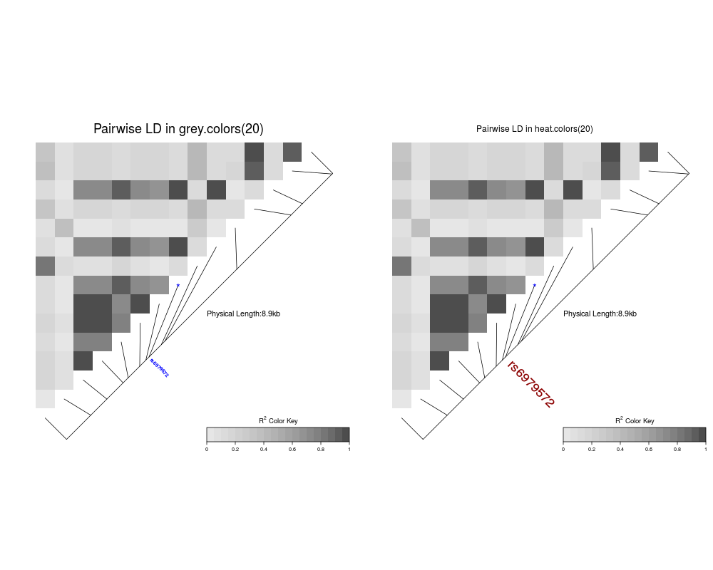
> ##Modify the text size of main title of the first heat map.
> grid.edit(gPath("ld1", "heatMap","title"), gp=gpar(cex=1.5))
>
> ##Modify the text size and color of the SNP label of the second heat map.
> grid.edit(gPath("ld2", "geneMap","SNPnames"), gp=gpar(cex=1.5, col="DarkRed"))
>
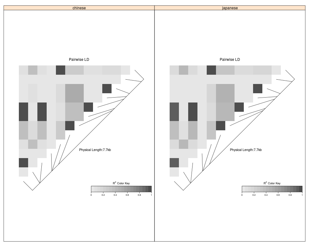
> #### Draw a lattice-like plot with heat maps in panels ####
> # Load CHBJPTSNP and CHBJPTDist
> data(CHBJPTData)
> # Make a variable which indicates Chinese vs. Japanese
> pop <- factor(c(rep("chinese",45), rep("japanese",45)))
> require(lattice)
Loading required package: lattice
>
> xyplot(1:nrow(CHBJPTSNP) ~ 1:nrow(CHBJPTSNP) | pop,
+ type="n", scales=list(draw=FALSE), xlab="", ylab="",
+ panel=function(x, y, subscripts,...) {
+ LDheatmap(CHBJPTSNP[subscripts,], CHBJPTDist, newpage=FALSE) })
>
> data(GIMAP5)
> require(lattice)
> n<-nrow(GIMAP5$snp.data)
> xyplot(1:n ~ 1:n | GIMAP5$subject.support$pop,
+ type="n", scales=list(draw=FALSE), xlab="", ylab="",
+ panel=function(x, y, subscripts,...) {
+ LDheatmap(GIMAP5$snp.data[subscripts,],
+ GIMAP5$snp.support$Position, SNP.name="rs6598", newpage=FALSE) })
>
>
>
> #Reset the user's setting for prompting on the graphics output
> #to the original value before running these example commands.
> devAskNewPage(old.prompt)
>
>
>
>
>
> dev.off()
null device
1
>
|