Supported by Dr. Osamu Ogasawara and  . . |
|
Last data update: 2014.03.03 |
Improved image() functionDescriptionImproved version of the The function Optionally Usage
image2(x = NULL, y = NULL, z = NULL, col = NULL, axes = FALSE, legend = TRUE,
    xlab = "", ylab = "", zlim = NULL, density = FALSE, max.height = NULL,
    zlim.label = "color scale", ...)

make_legend(data = NULL, col = NULL, side = 1, zlim = NULL, col.ticks = NULL,
    cex.axis = 2, max.height = 1, col.label = "")
Arguments
See Also
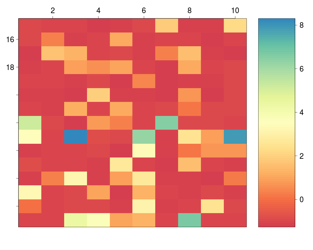
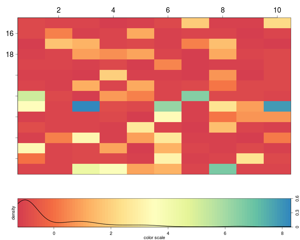
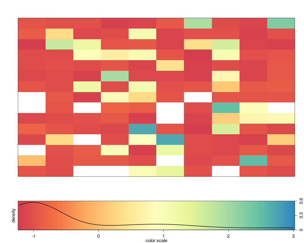
Examples## Not run: # Correlation matrix data(iris) # make sure its from 'datasets' package, not from 'locfit' image(cor(as.matrix(iris[, names(iris) != "Species"]))) # Correlation matrix has diagonal from top left to bottom right par(mar = c(1, 3, 1, 2)) image2(cor(as.matrix(iris[, names(iris) != "Species"])), col = "RdBu", axes = FALSE) ## End(Not run) # Color histogram nn <- 10 set.seed(nn) AA <- matrix(sample(c(rnorm(nn^2, -1, 0.1), rexp(nn^2/2, 0.5))), ncol = nn) image2(AA, col = "Spectral") image2(y = 1:15 + 2, x = 1:10, AA, col = "Spectral", axes = TRUE) image2(y = 1:15 + 2, x = 1:10, AA, col = "Spectral", density = TRUE, axes = TRUE) image2(AA, col = "Spectral", density = TRUE, zlim = c(min(AA), 3)) Results
R version 3.3.1 (2016-06-21) -- "Bug in Your Hair"
Copyright (C) 2016 The R Foundation for Statistical Computing
Platform: x86_64-pc-linux-gnu (64-bit)

R is free software and comes with ABSOLUTELY NO WARRANTY.
You are welcome to redistribute it under certain conditions.
Type 'license()' or 'licence()' for distribution details.

R is a collaborative project with many contributors.
Type 'contributors()' for more information and
'citation()' on how to cite R or R packages in publications.

Type 'demo()' for some demos, 'help()' for on-line help, or
'help.start()' for an HTML browser interface to help.
Type 'q()' to quit R.

> library(LICORS)
> png(filename="/home/ddbj/snapshot/RGM3/R_CC/result/LICORS/image2.Rd_%03d_medium.png", width=480, height=480)
> ### Name: image2
> ### Title: Improved image() function
> ### Aliases: image2 make_legend
> ### Keywords: aplot color hplot
>
> ### ** Examples
>
> ## Not run:
> ##D # Correlation matrix
> ##D data(iris)  # make sure its from 'datasets' package, not from 'locfit'
> ##D image(cor(as.matrix(iris[, names(iris) != "Species"])))
> ##D
> ##D # Correlation matrix has diagonal from top left to bottom right
> ##D par(mar = c(1, 3, 1, 2))
> ##D image2(cor(as.matrix(iris[, names(iris) != "Species"])), col = "RdBu", axes = FALSE)
> ## End(Not run)
> # Color histogram
> nn <- 10
> set.seed(nn)
> AA <- matrix(sample(c(rnorm(nn^2, -1, 0.1), rexp(nn^2/2, 0.5))), ncol = nn)
>
> image2(AA, col = "Spectral")
> image2(y = 1:15 + 2, x = 1:10, AA, col = "Spectral", axes = TRUE)
> image2(y = 1:15 + 2, x = 1:10, AA, col = "Spectral", density = TRUE, axes = TRUE)
>
> image2(AA, col = "Spectral", density = TRUE, zlim = c(min(AA), 3))
>
>
>
>
>
> dev.off()
null device
          1
>
|