Setup light cone geometry

Description

setup_LC_geometry sets up the light cone geometry for LICORS.

Usage

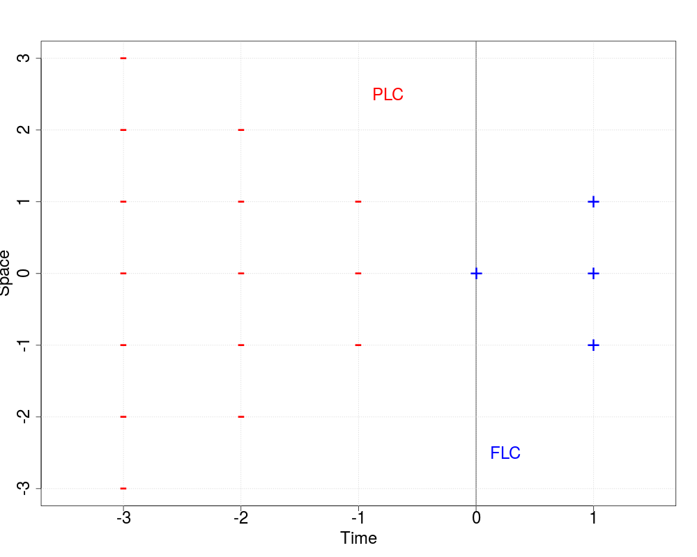
setup_LC_geometry(horizon = list(PLC = 1, FLC = 0), speed = 1, space.dim = 1, 
    shape = "cone")

Arguments

Value

A list of class "LC".

See Also

LC-utils, compute_LC_coordinates

Examples

aa <- setup_LC_geometry(horizon = list(PLC = 3, FLC = 1), speed = 1, space.dim = 1, 
    shape = "cone")
aa
plot(aa)
summary(aa)

Results

R version 3.3.1 (2016-06-21) -- "Bug in Your Hair"
Copyright (C) 2016 The R Foundation for Statistical Computing
Platform: x86_64-pc-linux-gnu (64-bit)

R is free software and comes with ABSOLUTELY NO WARRANTY.
You are welcome to redistribute it under certain conditions.
Type 'license()' or 'licence()' for distribution details.

R is a collaborative project with many contributors.
Type 'contributors()' for more information and
'citation()' on how to cite R or R packages in publications.

Type 'demo()' for some demos, 'help()' for on-line help, or
'help.start()' for an HTML browser interface to help.
Type 'q()' to quit R.

> library(LICORS)
> png(filename="/home/ddbj/snapshot/RGM3/R_CC/result/LICORS/setup_LC_geometry.Rd_%03d_medium.png", width=480, height=480)
> ### Name: setup_LC_geometry
> ### Title: Setup light cone geometry
> ### Aliases: setup_LC_geometry
> ### Keywords: manip
> 
> ### ** Examples
> 
> aa <- setup_LC_geometry(horizon = list(PLC = 3, FLC = 1), speed = 1, space.dim = 1, 
+     shape = "cone")
> aa
$horizon
$horizon$PLC
[1] 3

$horizon$FLC
[1] 1


$speed
[1] 1

$space.dim
[1] 1

$shape
[1] "cone"

$coordinates
$coordinates$PLC
      time x1
 [1,]   -1 -1
 [2,]   -1  0
 [3,]   -1  1
 [4,]   -2 -2
 [5,]   -2 -1
 [6,]   -2  0
 [7,]   -2  1
 [8,]   -2  2
 [9,]   -3 -3
[10,]   -3 -2
[11,]   -3 -1
[12,]   -3  0
[13,]   -3  1
[14,]   -3  2
[15,]   -3  3

$coordinates$FLC
     time x1
[1,]    0  0
[2,]    1 -1
[3,]    1  0
[4,]    1  1


$n.p
[1] 15

$n.f
[1] 4

attr(,"class")
[1] "LC"
> plot(aa)
> summary(aa)
   PLC  FLC
1    3    1
2    1    1
3 cone cone
4   15    4
* * * * * * * * * * * * * * * * * * * *
 
The field extends over a 1-dimensional space. 
Light cones have therefore the following characteristics: 
 
                PLC  FLC
horizon           3    1
speed             1    1
shape          cone cone
dimensionality   15    4

* * * * * * * * * * * * * * * * * * * *> 
> 
> 
> 
> 
> dev.off()
null device 
          1 
>