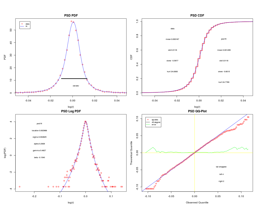
Poisson Subordinated Distribution

Description

A new Poisson subordinated distribution is proposed to capture major leptokurtic features in log-return time series of financial data. This distribution is intuitive, easy to calculate, and converge quickly. It fits well to the historical daily log-return distributions of currencies, commodities, Treasury yields, VIX, and, most difficult of all, DJIA. It serves as a viable alternative to the more sophisticated truncated stable distribution.

Author(s)

Stephen Horng-Twu Lihn <stevelihn@gmail.com>

References

On a Poisson Subordinated Distribution for Precise Statistical Measurement of Leptokurtic Financial Data, SSRN 2032762, http://papers.ssrn.com/sol3/papers.cfm?abstract_id=2032762.

See Also

dji_logr, rawmean, rawdensity, LIHNPSD_prepare_data, LIHNPSD_theoretical_result, LIHNPSD_plot_std4gr

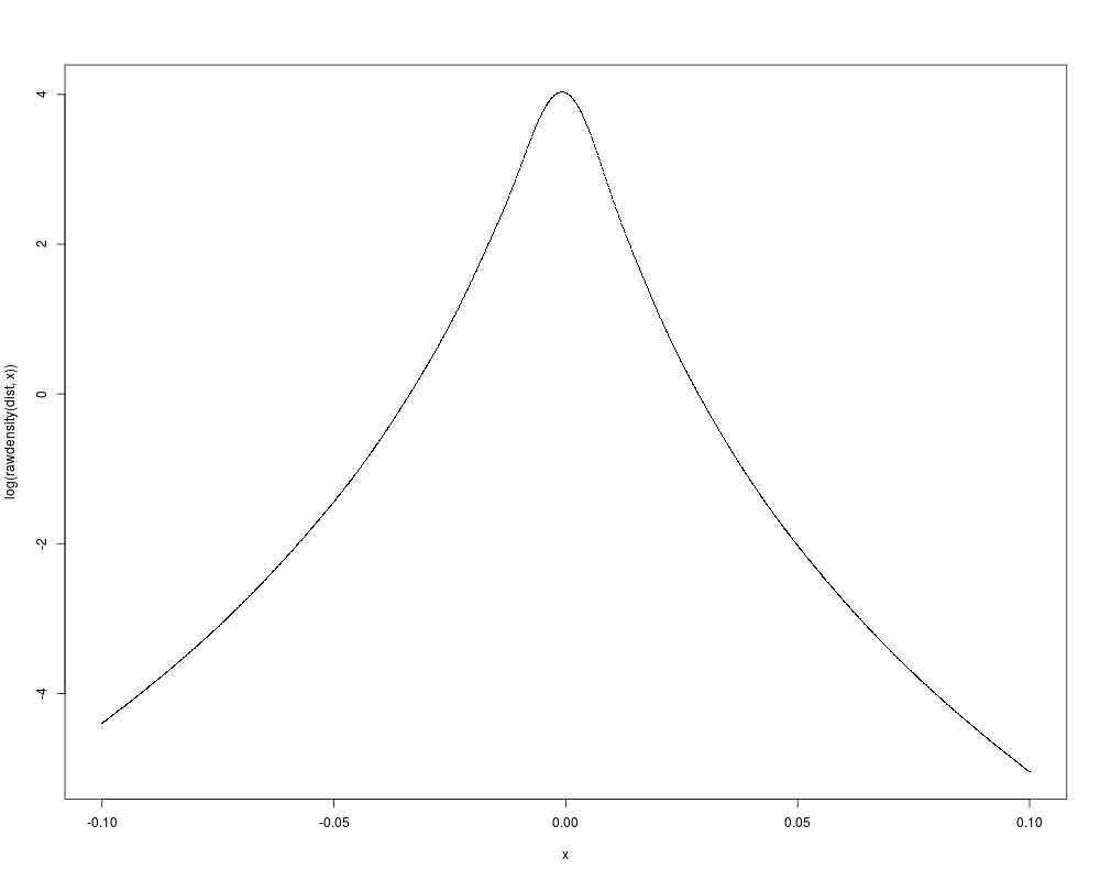
Examples

  # Load the daily log-return data of DJIA 
  data(dji_logr)
  
  # Construct the S3 object for PSD
  dist <- list( sigma= 0.004625, alpha= 0.292645, gamma= 0.482744, beta= -0.154049, location= 0.002968 )
  class(dist) <- "LIHNPSD"
  dist <- rawmean(dist)

  # A simple graph of the distribution's log PDF
  x <- seq(-0.1,0.1,by=0.1/1000)
  plot( x, log(rawdensity(dist,x)), pch=".")
  
  # The more sophisticated fit and graphs
  dt <- LIHNPSD_prepare_data(dji_logr, breaks=160, merge_tails=c(4,2))
  th <- LIHNPSD_theoretical_result(dist, dt)
  LIHNPSD_plot_std4gr(th, dt)

Results

R version 3.3.1 (2016-06-21) -- "Bug in Your Hair"
Copyright (C) 2016 The R Foundation for Statistical Computing
Platform: x86_64-pc-linux-gnu (64-bit)

R is free software and comes with ABSOLUTELY NO WARRANTY.
You are welcome to redistribute it under certain conditions.
Type 'license()' or 'licence()' for distribution details.

R is a collaborative project with many contributors.
Type 'contributors()' for more information and
'citation()' on how to cite R or R packages in publications.

Type 'demo()' for some demos, 'help()' for on-line help, or
'help.start()' for an HTML browser interface to help.
Type 'q()' to quit R.

> library(LIHNPSD)
Loading required package: sn
Loading required package: stats4

Attaching package: 'sn'

The following object is masked from 'package:stats':

    sd

Loading required package: moments
Loading required package: BB
Loading required package: Bolstad2
Loading required package: optimx
Loading required package: Rmpfr
Loading required package: gmp

Attaching package: 'gmp'

The following objects are masked from 'package:base':

    %*%, apply, crossprod, matrix, tcrossprod

C code of R package 'Rmpfr': GMP using 64 bits per limb


Attaching package: 'Rmpfr'

The following object is masked from 'package:sn':

    zeta

The following objects are masked from 'package:stats':

    dbinom, dnorm, dpois, pnorm

The following objects are masked from 'package:base':

    cbind, pmax, pmin, rbind


Attaching package: 'LIHNPSD'

The following object is masked from 'package:stats':

    density

> png(filename="/home/ddbj/snapshot/RGM3/R_CC/result/LIHNPSD/LIHNPSD-package.Rd_%03d_medium.png", width=480, height=480)
> ### Name: LIHNPSD-package
> ### Title: Poisson Subordinated Distribution
> ### Aliases: LIHNPSD-package LIHNPSD
> ### Keywords: package
> 
> ### ** Examples
> 
>   # Load the daily log-return data of DJIA 
>   data(dji_logr)
>   
>   # Construct the S3 object for PSD
>   dist <- list( sigma= 0.004625, alpha= 0.292645, gamma= 0.482744, beta= -0.154049, location= 0.002968 )
>   class(dist) <- "LIHNPSD"
>   dist <- rawmean(dist)
> 
>   # A simple graph of the distribution's log PDF
>   x <- seq(-0.1,0.1,by=0.1/1000)
>   plot( x, log(rawdensity(dist,x)), pch=".")
>   
>   # The more sophisticated fit and graphs
>   dt <- LIHNPSD_prepare_data(dji_logr, breaks=160, merge_tails=c(4,2))
>   th <- LIHNPSD_theoretical_result(dist, dt)
[1] "qqp tm1= 0.00 tm2= 0.01 tm3= 2.41 cdfcnt= 635"
>   LIHNPSD_plot_std4gr(th, dt)
> 
> 
> 
> 
> 
> dev.off()
null device 
          1 
>