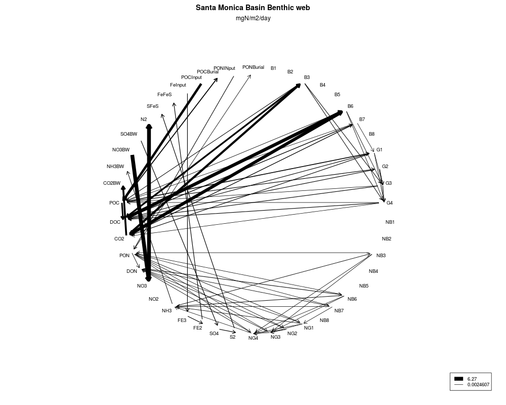
Linear inverse model specification for the Santa Monica Basin sediment food web

Description

Linear inverse model specification for the Santa Monica Basin (California) sediment food web as in Eldridge and Jackson (1993).

The Santa Monica Basin is a hypoxic-anoxic basin located near California.

The model contains both chemical and biological species.

The foodweb comprises 7 functional compartments and five external compartments, connected with 32 flows.

Units of the flows are mg /m2/day

The linear inverse model LIMCaliforniaSediment is generated from the file ‘CaliforniaSediment.input’ which can be found in subdirectory /examples/FoodWeb of the package directory

In this subdirectory you will find many foodweb example input files

These files can be read using Read and their output processed by Setup which will produce a linear inverse problem specification similar to LIMCaliforniaSediment

Usage

data(LIMCaliforniaSediment)

Format

a list of matrices, vectors, names and values that specify the linear inverse model problem.

see the return value of Setup for more information about this list

A more complete description of this structures is in vignette("LIM")

Author(s)

Karline Soetaert <karline.soetaert@nioz.nl> Dick van Oevelen <dick.vanoevelen@nioz.nl>

References

Eldridge, P.M., Jackson, G.A., 1993. Benthic trophic dynamics in California coastal basin and continental slope communities inferred using inverse analysis. Marine Ecology Progress Series 99, 115-135.

See Also

browseURL(paste(system.file(package="LIM"), "/doc/examples/Foodweb/", sep=""))

contains "CaliforniaSediment.input", the input file; read this with Setup

LIMTakapoto, LIMRigaSummer and many others

Examples

CaliforniaSediment <- Flowmatrix(LIMCaliforniaSediment)
plotweb(CaliforniaSediment, main = "Santa Monica Basin Benthic web",
        sub = "mgN/m2/day", lab.size = 0.8)
## Not run: 
xr <- LIMCaliforniaSediment$NUnknowns
i1 <- 1:(xr/2)
i2 <- (xr/2+1):xr
Plotranges(LIMCaliforniaSediment, index = i1, lab.cex = 0.7,
        sub = "*=unbounded",
        main = "Santa Monica Basin Benthic web, Flowranges - part1")
Plotranges(LIMCaliforniaSediment, index = i2, lab.cex = 0.7,
        sub = "*=unbounded",
        main = "Santa Monica Basin Benthic web, Flowranges - part2")
## End(Not run)

Results

R version 3.3.1 (2016-06-21) -- "Bug in Your Hair"
Copyright (C) 2016 The R Foundation for Statistical Computing
Platform: x86_64-pc-linux-gnu (64-bit)

R is free software and comes with ABSOLUTELY NO WARRANTY.
You are welcome to redistribute it under certain conditions.
Type 'license()' or 'licence()' for distribution details.

R is a collaborative project with many contributors.
Type 'contributors()' for more information and
'citation()' on how to cite R or R packages in publications.

Type 'demo()' for some demos, 'help()' for on-line help, or
'help.start()' for an HTML browser interface to help.
Type 'q()' to quit R.

> library(LIM)
Loading required package: limSolve
Loading required package: diagram
Loading required package: shape
> png(filename="/home/ddbj/snapshot/RGM3/R_CC/result/LIM/LIMCaliforniaSediment.Rd_%03d_medium.png", width=480, height=480)
> ### Name: LIMCaliforniaSediment
> ### Title: Linear inverse model specification for the Santa Monica Basin
> ###   sediment food web
> ### Aliases: LIMCaliforniaSediment
> ### Keywords: datasets
> 
> ### ** Examples
> 
> CaliforniaSediment <- Flowmatrix(LIMCaliforniaSediment)
> plotweb(CaliforniaSediment, main = "Santa Monica Basin Benthic web",
+         sub = "mgN/m2/day", lab.size = 0.8)
> ## Not run: 
> ##D xr <- LIMCaliforniaSediment$NUnknowns
> ##D i1 <- 1:(xr/2)
> ##D i2 <- (xr/2+1):xr
> ##D Plotranges(LIMCaliforniaSediment, index = i1, lab.cex = 0.7,
> ##D         sub = "*=unbounded",
> ##D         main = "Santa Monica Basin Benthic web, Flowranges - part1")
> ##D Plotranges(LIMCaliforniaSediment, index = i2, lab.cex = 0.7,
> ##D         sub = "*=unbounded",
> ##D         main = "Santa Monica Basin Benthic web, Flowranges - part2")
> ## End(Not run)
> 
> 
> 
> 
> 
> dev.off()
null device 
          1 
>