The function returns a plot after fitting a dataset to a given equation.
Usage
## S3 method for class 'plot'
AQSys(XYdt, xlbl = "", ylbl = "", main = NULL,
  col = "blue", type = "p", cex = 1, cexlab = 1, cexaxis = 1,
  cexmain = 1, cexsub = 1, xmax = 0.4, ymax = 0.5, HR = FALSE,
  NP = 100, mathDesc = "merchuk", clwd = NULL, save = FALSE, ...)
Arguments
XYdt
Binodal Experimental data that will be used in the nonlinear fit
xlbl
Plot's Horizontal axis label.
ylbl
Plot's Vertical axis label.
main
Legacy from plot package. For more details, see plot.default
col
Legacy from plot package. For more details, see plot.default
type
Legacy from plot package. For more details, see plot.default
cex
Legacy from plot package. For more details, see plot.default
cexlab
Legacy from plot package. For more details, see plot.default
cexaxis
Legacy from plot package. For more details, see plot.default
cexmain
Legacy from plot package. For more details, see plot.default
cexsub
Legacy from plot package. For more details, see plot.default
xmax
Maximum value for the Horizontal axis' value
ymax
Maximum value for the Vertical axis' value
HR
Magnify Plot's text to be compatible with High Resolution size [type:Boulean]
NP
Number of points used to build the fitted curve. Default is 100. [type:Integer]
mathDesc
- Character String specifying the nonlinear empirical equation to fit data. The default method uses
Merchuk's equation. Other possibilities can be seen in AQSysList().
clwd
Plot's axis line width
save
Optimize Plot's elements to be compatible with High Resolution size [type:Boulean]
...
Additional optional arguments. None are used at present.
Details
This version uses the plot function and return a regular bidimensional plot.
Value
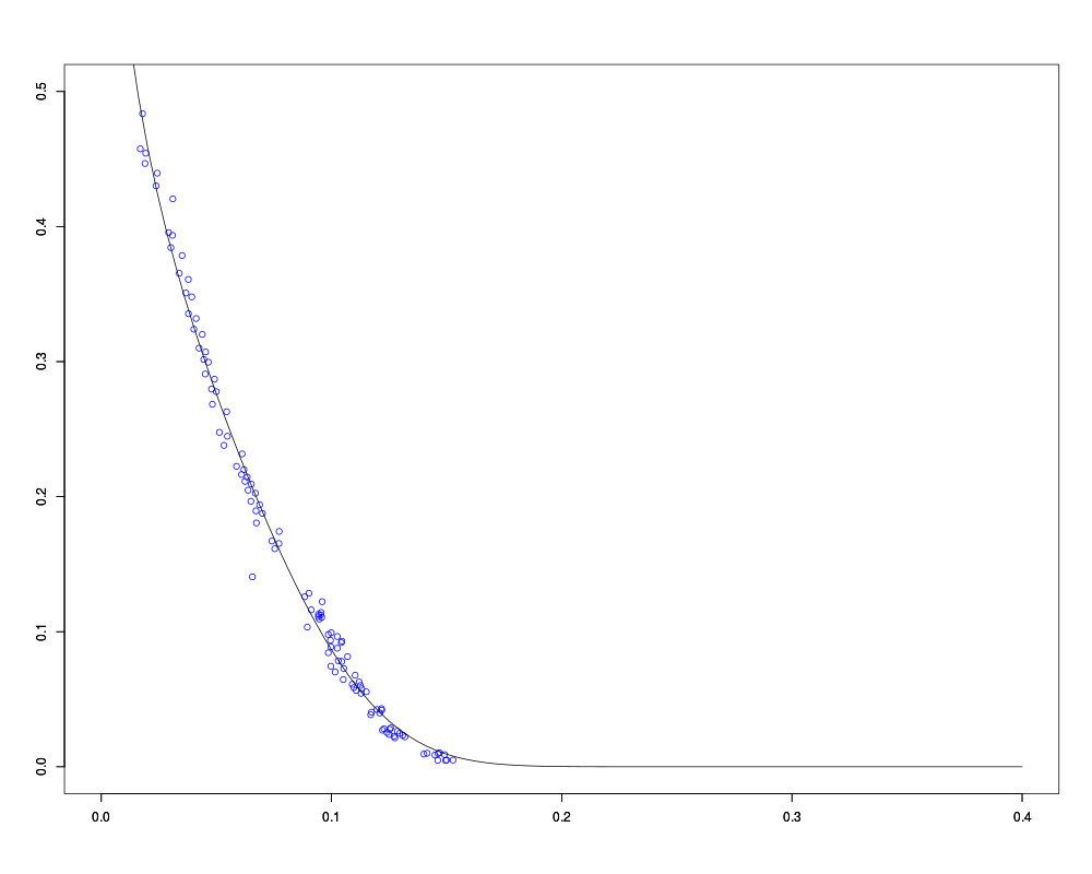
A plot containing the experimental data, the correspondent curve for the binodal in study and the curve's raw XY data.
Examples
#Populating variable XYdt with binodal data
XYdt <- peg4kslt[,1:2]
#Plot XYdt using Merchuk's function
#
AQSys.plot(XYdt)
#
Results
R version 3.3.1 (2016-06-21) -- "Bug in Your Hair"
Copyright (C) 2016 The R Foundation for Statistical Computing
Platform: x86_64-pc-linux-gnu (64-bit)

R is free software and comes with ABSOLUTELY NO WARRANTY.
You are welcome to redistribute it under certain conditions.
Type 'license()' or 'licence()' for distribution details.

R is a collaborative project with many contributors.
Type 'contributors()' for more information and
'citation()' on how to cite R or R packages in publications.

Type 'demo()' for some demos, 'help()' for on-line help, or
'help.start()' for an HTML browser interface to help.
Type 'q()' to quit R.

> library(LLSR)
Loading required package: rootSolve
Loading required package: XLConnect
Loading required package: XLConnectJars
XLConnect 0.2-12 by Mirai Solutions GmbH [aut],
  Martin Studer [cre],
  The Apache Software Foundation [ctb, cph] (Apache POI, Apache Commons
    Codec),
  Stephen Colebourne [ctb, cph] (Joda-Time Java library),
  Graph Builder [ctb, cph] (Curvesapi Java library)
http://www.mirai-solutions.com ,
http://miraisolutions.wordpress.com
Loading required package: digest
Loading required package: svDialogs
Loading required package: svGUI
Loading required package: ggtern
Loading required package: ggplot2

Attaching package: 'ggtern'

The following objects are masked from 'package:ggplot2':

    aes, calc_element, ggplot, ggplotGrob, ggplot_build, ggplot_gtable,
    ggsave, is.ggplot, layer_data, layer_grob, layer_scales, theme,
    theme_bw, theme_classic, theme_dark, theme_get, theme_gray,
    theme_light, theme_linedraw, theme_minimal, theme_set, theme_void


    Be aware that LLSR is a collaborative package that still in
    development and your help is essential.

    If you found any bugs or have a suggestion, do not hesitate and
    contact us on https://github.com/eqipehub/LLSR/issues.

    You also can fork this project directly from github and commit
    improvements to us (https://github.com/eqipehub/LLSR).

    The information used in the database was obtained free of charge
    but it might be copyrighted by third parties and references must
    be included appropriately.

    Please use LLSR.info() to read more details about the current
    package version.
> png(filename="/home/ddbj/snapshot/RGM3/R_CC/result/LLSR/AQSys.plot.Rd_%03d_medium.png", width=480, height=480)
> ### Name: AQSys.plot
> ### Title: Dataset and Fitted Function plot
> ### Aliases: AQSys.plot
>
> ### ** Examples
>
> #Populating variable XYdt with binodal data
> XYdt <- peg4kslt[,1:2]
> #Plot XYdt using Merchuk's function
> #
> AQSys.plot(XYdt)
> #
>
>
>
>
>
> dev.off()
null device
          1
>
 .
.