R Graphical Manual

Browse All

Last data update: 2014.03.03

R: Coverage and self-coverage plots.

coverage

R Documentation

Coverage and self-coverage plots.

Description

These functions compute coverages (for any principal object), and self-coverages (only for local principal curves, these may be used for bandwidth selection).

Usage

coverage.raw(X, vec, tau, weights=1, plot.type="p", print=FALSE,
      label=NULL,...)

coverage(X, vec, taumin=0.02, taumax, gridsize=25, weights=1,
      plot.type="o", print=FALSE,...)

lpc.coverage(object, taumin=0.02, taumax, gridsize=25, quick=TRUE,
      plot.type="o", print=FALSE, ...)

lpc.self.coverage(X,  taumin=0.02, taumax=0.5,   gridsize=25, x0=1,
     way = "two", scaled=TRUE,  weights=1, pen=2, depth=1,
     control=lpc.control(boundary=0, cross=FALSE),   quick=TRUE,
     plot.type="o", print=FALSE, ... )

select.self.coverage(self,  smin, plot.type="o", plot.segments=NULL)

Arguments

`X`	a N x d data matrix.
`object`	An object of type `lpc` or `lpc.spline`.
`vec`	A matrix with d columns. The rows contain the points which make up the fitted object.
`tau`	tube size.
`taumin`	Minimal tube size.
`taumax`	Maximal tube size.
`weights`	An optional vector of weights. If weights are specified, then the coverage is the weighted mean of the indicator functions for falling within the tube. The function `lpc.coverage` does not have a `weights` argument, as it extracts the weights from the `$weights` component of the fitted `object`.
`label`	Experimental option; don't use.
`gridsize`	The number of different tube sizes to consider.
`quick`	If TRUE, an approximate coverage curve is provided by computing distances between data points and the curve through the closest local centers or mass; whereas with FALSE we use the distances of the points when projected orthogonally onto the spline representation of the local principal curve. The latter takes considerably more computing time. The resulting coverage curves are generally very similar, but the quick version may deliver little spurious peaks occasionally.
`self`	An object of class `self`, or a matrix with two colums providing a self-coverage curve.
`smin`	Minimum coverage for bandwidth selection. Default: 1/3 for clustering, 2/3 for principal curves.
`plot.type`	If set to 0, no plotted output is given. Otherwise, an appropriate plot is provided, using the plotting type as specified.
`plot.segments`	A list with default `list(lty=c(1,2,3), lwd=c(2,1,1),lcol=c(3,3,3))` which specifies how (and how many) bandwidth candidates, in order of decreasing negative second derivative of self-coverage, are to be highlighted.
`print`	If TRUE, coverage values are printed on the screen as soon as computed. This is quite helpful especially if `gridsize` is large.
`x0, way, scaled, pen, depth, control`	LPC parameters as outlined in `lpc` and `lpc.control`.
`...`	Optional graphical parameters passed to the corresponding plotting functions.

Details

The function coverage.raw computes the coverage, i.e. the proportion of data points lying inside a circle or band with radius tau, for a fixed value tau. The whole coverage curve C(tau) is constructed through function coverage.

Functions coverage.raw and coverage can be used for any object fitted by an unsupervised learning technique (for instance, HS principal curves, or even clustering algorithms), while the functions prefixing with lpc. can only be used for local principal curves. The function lpc.coverage is a wrapper around coverage which takes directly a fitted lpc object, rather than a data matrix.

Function select.self.coverage extracts suitable bandwidths from the self-coverage curve, and produces a plot. The function is called from within lpc.self.coverage, but can also be called directly by the user (for instance, if the graphical output is to be reproduced, or if the minimum coverage smin is to be modified). The component $select contains the selected candidate bandwidths, in the order of strength of evidence provided by the self-coverage criterion (the best bandwidth comes first, etc.). A plot is produced as a by-product, which symbolizes the best bandwidth by a thick solid line, the second-best by a dashed line, and the third-best by a dotted line. It is recommended to run the self-coverage functions with fixed starting points, as in the examples below.

See Einbeck (2011) for details. Note that the original publication by Einbeck, Tutz, and Evers (2005) uses ‘quick’ coverage curves.

Value

A list of items, and a plot (unless plot.type=0).

The function lpc.self.coverage produces an object of class self. The component $select recommends suitable bandwidths for the use in lpc, in the order of strength of evidence. These correspond to points of strong negative curvature (implemented via second differences) of the self-coverage curve.

Author(s)

J. Einbeck

References

Einbeck, J., Tutz, G., & Evers, L. (2005). Local principal curves. Statistics and Computing 15, 301-313.

Einbeck, J. (2011). Bandwidth selection for mean-shift based unsupervised learning techniques: a unified approach via self-coverage. Journal of Pattern Recognition Research 6, 175-192.

Examples

data(gvessel)
## Not run: gvessel.self <-lpc.self.coverage(gvessel[,c(2,4,5)], x0=c(35, 1870,
6.3), print=FALSE, plot.type=0)
h <- select.self.coverage(gvessel.self)$select
gvessel.lpc <- lpc(gvessel[,c(2,4,5)], h=h[1],  x0=c(35, 1870, 6.3))
lpc.coverage(gvessel.lpc, gridsize=10, print=FALSE)

## End(Not run)

data(calspeedflow)
fitms <- ms(calspeedflow[,3:4])
coverage(fitms$data, fitms$cluster.center)

Results


R version 3.3.1 (2016-06-21) -- "Bug in Your Hair"
Copyright (C) 2016 The R Foundation for Statistical Computing
Platform: x86_64-pc-linux-gnu (64-bit)

R is free software and comes with ABSOLUTELY NO WARRANTY.
You are welcome to redistribute it under certain conditions.
Type 'license()' or 'licence()' for distribution details.

R is a collaborative project with many contributors.
Type 'contributors()' for more information and
'citation()' on how to cite R or R packages in publications.

Type 'demo()' for some demos, 'help()' for on-line help, or
'help.start()' for an HTML browser interface to help.
Type 'q()' to quit R.

> library(LPCM)
> png(filename="/home/ddbj/snapshot/RGM3/R_CC/result/LPCM/coverage.Rd_%03d_medium.png", width=480, height=480)
> ### Name: coverage
> ### Title: Coverage and self-coverage plots.
> ### Aliases: coverage coverage.raw lpc.coverage lpc.self.coverage
> ###   select.self.coverage
> ### Keywords: multivariate
> 
> ### ** Examples
> 
> data(gvessel)
> ## Not run: 
> ##D gvessel.self <-lpc.self.coverage(gvessel[,c(2,4,5)], x0=c(35, 1870,
> ##D 6.3), print=FALSE, plot.type=0)
> ##D h <- select.self.coverage(gvessel.self)$select
> ##D gvessel.lpc <- lpc(gvessel[,c(2,4,5)], h=h[1],  x0=c(35, 1870, 6.3))
> ##D lpc.coverage(gvessel.lpc, gridsize=10, print=FALSE)
> ## End(Not run)
> 
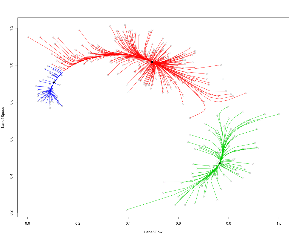
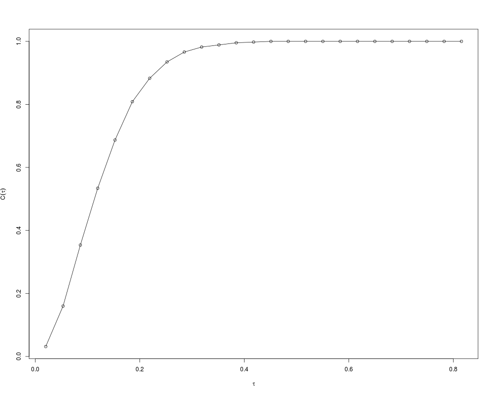
> data(calspeedflow)
> fitms <- ms(calspeedflow[,3:4])
> coverage(fitms$data, fitms$cluster.center)
$tau
 [1] 0.02000000 0.05314603 0.08629205 0.11943808 0.15258410 0.18573013
 [7] 0.21887615 0.25202218 0.28516820 0.31831423 0.35146026 0.38460628
[13] 0.41775231 0.45089833 0.48404436 0.51719038 0.55033641 0.58348243
[19] 0.61662846 0.64977448 0.68292051 0.71606654 0.74921256 0.78235859
[25] 0.81550461

$coverage
 [1] 0.03153153 0.15990991 0.35360360 0.53378378 0.68693694 0.80855856
 [7] 0.88288288 0.93468468 0.96621622 0.98198198 0.98873874 0.99549550
[13] 0.99774775 1.00000000 1.00000000 1.00000000 1.00000000 1.00000000
[19] 1.00000000 1.00000000 1.00000000 1.00000000 1.00000000 1.00000000
[25] 1.00000000

> 
> 
> 
> 
> 
> dev.off()
null device 
          1 
>