R Graphical Manual

Browse All

Last data update: 2014.03.03

R: Local principal curves

lpc	R Documentation

Local principal curves

Description

This is the main function which computes the actual local principal curve, i.e. a sequence of local centers of mass.

Usage

lpc(X, h, t0 = mean(h),  x0,  way = "two",  scaled = TRUE,
      weights=1, pen = 2, depth = 1, control=lpc.control())

Arguments

`X`	data matrix with N rows (observations) and d columns (variables).
`h`	bandwidth. May be either specified as a single number, then the same bandwidth is used in all dimensions, or as a d-dimensional bandwidth vector. The default setting is 10 percent of the range in each direction. If `scaled =TRUE` then the bandwidth has to be specified in fractions of the data range, e.g. h= c(0.2,0.1), rather than absolute values.
`t0`	scalar step length. Default setting is `t0=h`, if `h` is a scalar, and `t0=mean(h)`, if `h` is a vector.
`x0`	specifies the choice of starting points. The default choice `x0=1` will select one suitable starting point automatically (in form of a local density mode). The second built-in option `x0=0` will use all local density modes as starting points, hence produce as many branches as modes. Optionally, one can also set one or more starting points manually here. This can be done in form of a matrix, where each row corresponds to a starting point, or in form of a vector, where starting points are read in consecutive order from the entries of the vector. The starting point has always to be specified on the original data scale, even if `scaled=TRUE`. A fixed number of starting points can be enforced through option `mult` in `lpc.control`.
`way`	"one": go only in direction of the first local eigenvector, "back": go only in opposite direction, "two": go from starting point in both directions.
`scaled`	if TRUE, scales each variable by dividing through its range (see also the Notes section below).
`weights`	a vector of observation weights (can also be used to exclude individual observations from the computation by setting their weight to zero.)
`pen`	power used for angle penalization (see [1]). If set to 0, the angle penalization is switched off.
`depth`	maximum depth of branches (phi_max in [2]), restricted to the values 1,2 or 3 (The original LPC branch has depth 1. If, along this curve, a point features a high second local PC, this launches a new starting point, and the resulting branch has depth 2. If, along this branch, a point features a high second local PC, this launches a new starting point, and the resulting branch has depth 3. )
`control`	Additional parameters steering particularly the starting-, boundary-, and convergence behavior of the fitted curve. See `lpc.control`.

Value

A list of items:

`LPC`	The coordinates of the local centers of mass of the fitted principal curve.
`Parametrization`	Curve parameters and branch labels for each local center of mass.
`h`	The bandwidth used for the curve estimation.
`to`	The constant t0 used for the curve estimation.
`starting.points`	The coordinates of the starting point(s) used.
`data`	The data frame used for curve estimation.
`scaled`	Logical.
`weights`	The vector of weights used for curve estimation.
`control`	The settings used in `lpc.control()`
`Misc`	Miscellannea.

Note

All values provided in the output refer to the scaled data, if scaled=TRUE. Use unscale to convert the results back to the original data scale.

The option scaled=TRUE scales the data by dividing each variable through their range. This differs from the usual scaling through the standard deviation as common for PCA, but we found the algorithm and the default bandwidth selection to work more reliably this way. If you wish to scale by the standard deviation, please do that by feeding the scaled data directly into the lpc function, i.e.

lpc(sweep(data, 2,sd(data), "/"),h, t0, ..., scaled=FALSE, ...).

Author(s)

J. Einbeck and L. Evers. See LPCM-package for further acknowledgements.

References

[1] Einbeck, J., Tutz, G., & Evers, L. (2005). Local principal curves. Statistics and Computing 15, 301-313.

[2] Einbeck, J., Tutz, G., & Evers, L. (2005): Exploring Multivariate Data Structures with Local Principal Curves. In: Weihs, C. and Gaul, W. (Eds.): Classification - The Ubiquitous Challenge. Springer, Heidelberg, pages 256-263.

Examples


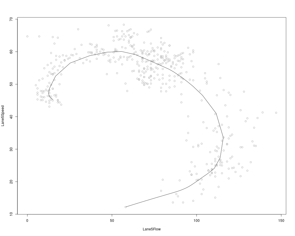
data(calspeedflow)
lpc1 <- lpc(calspeedflow[,3:4])
plot(lpc1)

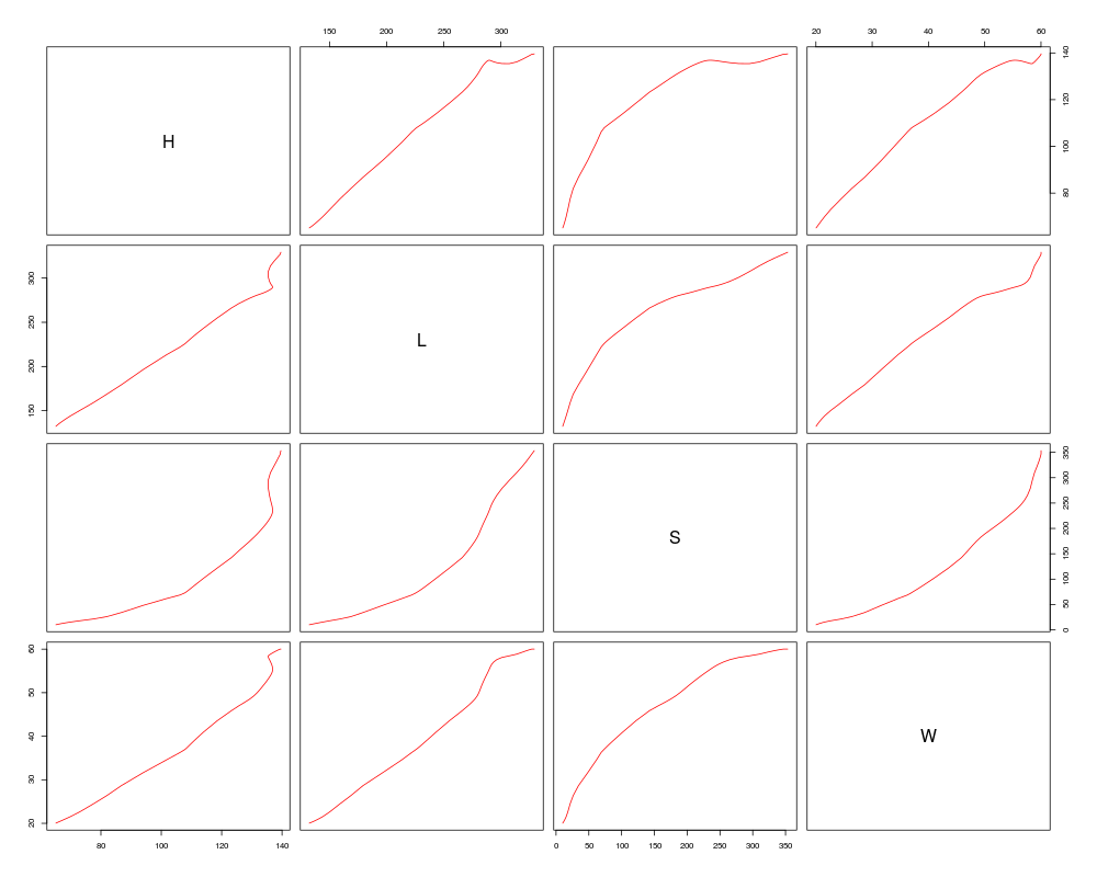
data(mussels, package="dr")
 lpc2 <- lpc(mussels[,-3], x0=as.numeric(mussels[49,-3]),scaled=FALSE)
 plot(lpc2, curvecol=2)

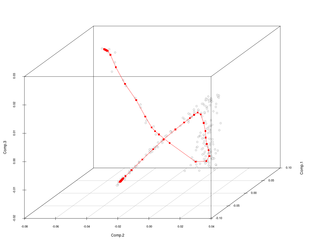
data(gaia)
s <- sample(nrow(gaia),200)
gaia.pc <-  princomp(gaia[s,5:20])
lpc3 <- lpc(gaia.pc$scores[,c(2,1,3)],scaled=FALSE)
plot(lpc3, curvecol=2, type=c("curve","mass"))

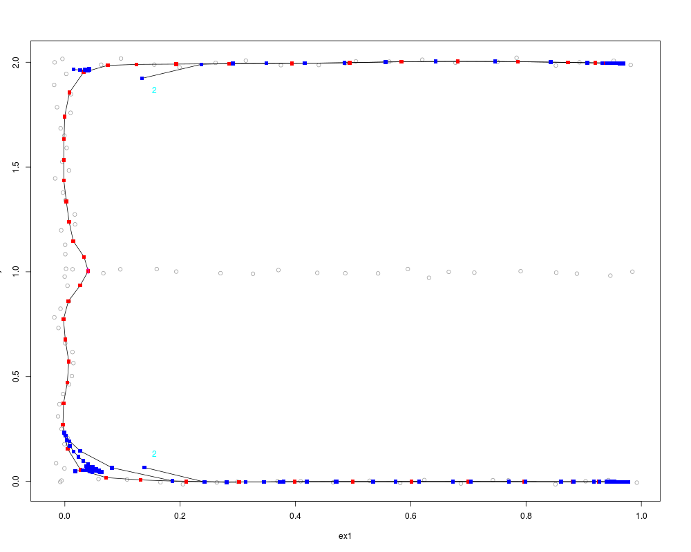
# Simulated letter 'E' with branched LPC
ex<- c(rep(0,40), seq(0,1,length=20), seq(0,1,length=20), seq(0,1,length=20))
ey<- c(seq(0,2,length=40), rep(0,20), rep(1,20), rep(2,20))
sex<-rnorm(100,0,0.01); sey<-rnorm(100,0,0.01)
eex<-rnorm(100,0,0.1);  eey<-rnorm(100,0,0.1)
ex1<-ex+sex; ey1<-ey+sey
ex2<-ex+eex; ey2<-ey+eey
e1<-cbind(ex1,ey1); e2<-cbind(ex2,ey2)
lpc.e1 <- lpc(e1, h= c(0.1,0.1),  depth=2, scaled=FALSE)
plot(lpc.e1, type=c("curve","mass", "start"))

Results


R version 3.3.1 (2016-06-21) -- "Bug in Your Hair"
Copyright (C) 2016 The R Foundation for Statistical Computing
Platform: x86_64-pc-linux-gnu (64-bit)

R is free software and comes with ABSOLUTELY NO WARRANTY.
You are welcome to redistribute it under certain conditions.
Type 'license()' or 'licence()' for distribution details.

R is a collaborative project with many contributors.
Type 'contributors()' for more information and
'citation()' on how to cite R or R packages in publications.

Type 'demo()' for some demos, 'help()' for on-line help, or
'help.start()' for an HTML browser interface to help.
Type 'q()' to quit R.

> library(LPCM)
> png(filename="/home/ddbj/snapshot/RGM3/R_CC/result/LPCM/lpc.Rd_%03d_medium.png", width=480, height=480)
> ### Name: lpc
> ### Title: Local principal curves
> ### Aliases: lpc
> ### Keywords: smooth multivariate
> 
> ### ** Examples
> 
> 
> data(calspeedflow)
> lpc1 <- lpc(calspeedflow[,3:4])
> plot(lpc1)
> 
> data(mussels, package="dr")
>  lpc2 <- lpc(mussels[,-3], x0=as.numeric(mussels[49,-3]),scaled=FALSE)
>  plot(lpc2, curvecol=2)
> 
> data(gaia)
> s <- sample(nrow(gaia),200)
> gaia.pc <-  princomp(gaia[s,5:20])
> lpc3 <- lpc(gaia.pc$scores[,c(2,1,3)],scaled=FALSE)
> plot(lpc3, curvecol=2, type=c("curve","mass"))
> 
> # Simulated letter 'E' with branched LPC
> ex<- c(rep(0,40), seq(0,1,length=20), seq(0,1,length=20), seq(0,1,length=20))
> ey<- c(seq(0,2,length=40), rep(0,20), rep(1,20), rep(2,20))
> sex<-rnorm(100,0,0.01); sey<-rnorm(100,0,0.01)
> eex<-rnorm(100,0,0.1);  eey<-rnorm(100,0,0.1)
> ex1<-ex+sex; ey1<-ey+sey
> ex2<-ex+eex; ey2<-ey+eey
> e1<-cbind(ex1,ey1); e2<-cbind(ex2,ey2)
> lpc.e1 <- lpc(e1, h= c(0.1,0.1),  depth=2, scaled=FALSE)
> plot(lpc.e1, type=c("curve","mass", "start"))
> 
> 
> 
> 
> 
> dev.off()
null device 
          1 
>