R Graphical Manual

Browse All

Last data update: 2014.03.03

R: Representing local principal curves through a cubic spline.

lpc.spline

R Documentation

Representing local principal curves through a cubic spline.

Description

Fis a natural cubic spline component-wise through the series of local centers of mass. This provides a continuous parametrization in terms of arc length distance, which can be used to compute a projection index for the original or new data points.

Usage

lpc.spline(lpcobject, optimize = TRUE, compute.Rc=FALSE,
     project=FALSE, ...)

Arguments

`lpcobject`	Object of class `lpc`.
`optimize`	Boolean. If TRUE, `optimize` is used to find the point on the curve with minimum distance. Otherwise, data points are only projected onto the closest knot.
`compute.Rc`	Boolean. If TRUE, the goodness-of-fit measure R_c suggested in [1] is computed and returned (using the scaled data, if `scaled=TRUE` in `lpcobject`).
`project`	Boolean. If TRUE, projections onto curve are computed.
`...`	Additional arguments to be passed to `lpc.project.spline`

Details

See reference [2].

Value

`knots.pi`	LPC parameters (in cubic spline parametrization) at position of the knots of the spline function (these are not identical to the LPC mass points!)
`knots.coords`	Coordinates of the spline knots.
`closest.pi`	Parameter of the projected data points.
`closest.coords`	Coordinates of projected data points.
`closest.dist`	Euclidean distance between original and projected data point.
`closest.branch`	ID Number of the branch on which the data point was projected (the IDs are given in the output of function `lpc`).
`Rc`	Value of R_c.
`project`	repeats the input value of `project`.
`lpcobject`	returns the provided object `lpcobject`.
`splinefun`	returns the cubic spline function (generated by `lpc.splinefun`).

Warning

Careful with options project and compute.Rc - they can take rather long if the data set is large!

Note

The parametrization of the cubic spline function is not exactly the same as that of the original LPC. The reason is that the latter uses Euclidean distances between centers of masses, while the former uses the arc length along the cubic spline. However, the differences are normally quite small.

Author(s)

J. Einbeck and L. Evers

References

[1] Einbeck, J., Tutz, G., and Evers, L. (2005). Local principal curves. Statistics and Computing 15, 301-313.

[2] Einbeck, J., Evers, L. & Hinchliff, K. (2010): Data compression and regression based on local principal curves. In A. Fink, B. Lausen, W. Seidel, and A. Ultsch (Eds), Advances in Data Analysis, Data Handling, and Business Intelligence, Heidelberg, pp. 701–712, Springer.

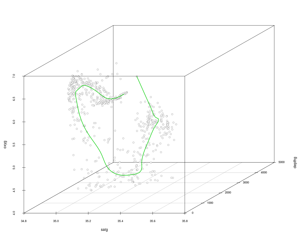
Examples

data(gvessel)
gvessel.lpc <- lpc(gvessel[,c(2,4,5)],   h=0.11,  x0=c(35, 1870, 6.3))
gvessel.spline  <- lpc.spline(gvessel.lpc)
plot(gvessel.spline, lwd=2)

Results


R version 3.3.1 (2016-06-21) -- "Bug in Your Hair"
Copyright (C) 2016 The R Foundation for Statistical Computing
Platform: x86_64-pc-linux-gnu (64-bit)

R is free software and comes with ABSOLUTELY NO WARRANTY.
You are welcome to redistribute it under certain conditions.
Type 'license()' or 'licence()' for distribution details.

R is a collaborative project with many contributors.
Type 'contributors()' for more information and
'citation()' on how to cite R or R packages in publications.

Type 'demo()' for some demos, 'help()' for on-line help, or
'help.start()' for an HTML browser interface to help.
Type 'q()' to quit R.

> library(LPCM)
> png(filename="/home/ddbj/snapshot/RGM3/R_CC/result/LPCM/lpc.spline.Rd_%03d_medium.png", width=480, height=480)
> ### Name: lpc.spline
> ### Title: Representing local principal curves through a cubic spline.
> ### Aliases: lpc.spline
> ### Keywords: smooth multivariate
> 
> ### ** Examples
> 
> data(gvessel)
> gvessel.lpc <- lpc(gvessel[,c(2,4,5)],   h=0.11,  x0=c(35, 1870, 6.3))
> gvessel.spline  <- lpc.spline(gvessel.lpc)
> plot(gvessel.spline, lwd=2)
> 
> 
> 
> 
> 
> dev.off()
null device 
          1 
>