R Graphical Manual

Browse All

Last data update: 2014.03.03

R: Mean shift clustering.

ms	R Documentation

Mean shift clustering.

Description

Functions for mean shift, iterative mean shift, mean shift clustering, and bandwidth selection for mean shift clustering (based on self-coverage). The main function is ms which, for a given bandwidth, detects the local modes (‘local principal points’) and performs the clustering.

These functions implement the techniques presented in Einbeck (2011).

Usage

meanshift(X, x, h)
ms.rep(X, x, h, plotms=1, thresh= 0.00000001, iter=200)
ms(X, h, subset,  thr=0.0001, scaled= TRUE, iter=200, plotms=2,
       or.labels=NULL, ...)
ms.self.coverage(X, taumin=0.02, taumax=0.5, gridsize=25,
       thr=0.0001, scaled=TRUE, cluster=FALSE, plot.type="o", 
       or.labels=NULL, print=FALSE, ...)

Arguments

`X`	data matrix.
`h`	bandwidth (by default, 10 percent of the data range).
`x`	point from which we wish to shift to the local mean.
`subset`	vector specifying a subset of 1:n, where n is the sample size. This allows to run the iterative mean shift procedure only from a subset of points (if unspecified, 1:n is used here, i.e. each data point serves as a starting point).
`scaled`	logical (if TRUE, each variable is divided by its range).
`taumin,taumax,gridsize`	determine the grid of bandwidths to investigate.
`thresh, iter`	mean shift iterations are stopped when the mean shift length (relative to the length of `x`) falls below `thresh`, or after `iter` iterations (whatever event happens first).
`thr`	adjacent mean shift clusters are merged if their relative distance falls below this threshold.
`cluster`	if `TRUE`, distances are always measured to the cluster to which an observation is assigned, rather than to the nearest cluster.
`plotms, plot.type, or.labels, ...`	graphical parameters.
`print`	if TRUE, coverage values are printed on the screen as soon as computed. This is quite helpful especially if `gridsize` is large.

Details

The methods implemented here can be used for density mode estimation, clustering, and the selection of starting points for the LPC algorithm.

Chen (1995) showed that, if the mean shift is computed iteratively, the resulting sequence of local means converges to a mode of the estimated density function. By assigning each data point to the mode to which it has converged, this turns into a clustering technique.

The concepts of coverage and self-coverage, which were originally introduced in the principal curve context, adapt straightforwardly to this setting.

The goodness-of-fit messure Rc can also be applied in this context. For instance, a value of R_C=0.8 means that, after the clustering, the mean absolute residual length has been reduced by 80% (compared to the distances to the overall mean).

Value

The main function ms produces an object of class ms, with components:

`cluster.center`	a matrix which gives the coordinates of the estimated density modes (i.e., of the mean-shift based cluster centers).
`cluster.label`	assigns each data point to the cluster center to which its mean shift trajectory has converged.
`closest.label`	assigns each data point to the closest cluster center in terms of Euclidean distance.
`data`	the data frame (scaled if `scaled=TRUE`).
`scaled`	boolean.
`scaled.by`	the data were scaled by dividing each variable through the values provided in this vector.

For all other functions, use names().

Author(s)

J. Einbeck. See LPCM-package for further acknowledgements.

References

Chen, Y. (1995). Mean Shift, Mode Seeking, and Clustering. IEEE Transactions on Pattern Analysis and Machine Intelligence, 17, 790-799.

Einbeck, J. (2011). Bandwidth selection for mean-shift based unsupervised learning techniques: a unified approach via self-coverage. Journal of Pattern Recognition Research 6, 175-192.

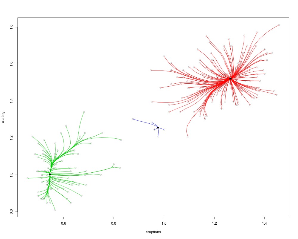
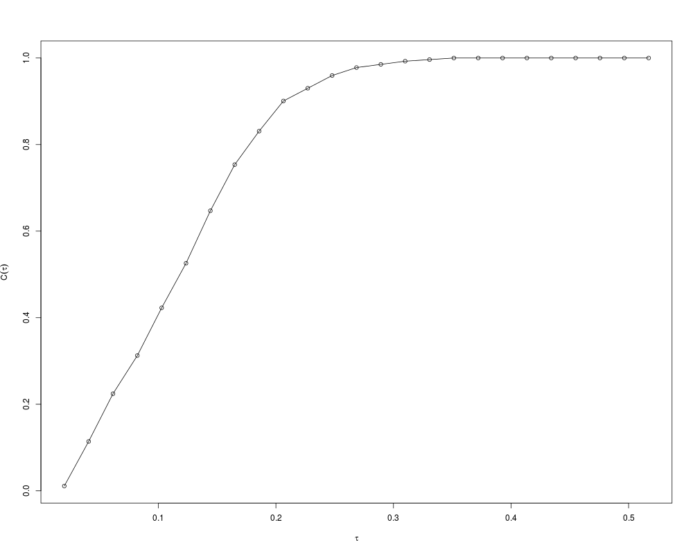
Examples

data(faithful)
# Mean shift clustering with user-defined bandwidth (5 percent of data range)
fit <- ms(faithful, h=0.05)

# Goodness-of-fit
coverage(fit$data, fit$cluster.center)
Rc(fit)

# Bandwidth selection via self-coverage
## Not run: foo <- ms.self.coverage(faithful,gridsize= 50, taumin=0.1,
taumax=0.5, plot.type="o")   
h <- select.self.coverage(foo)$select
fit <- ms(faithful,h=h[1])
## End(Not run)

Results


R version 3.3.1 (2016-06-21) -- "Bug in Your Hair"
Copyright (C) 2016 The R Foundation for Statistical Computing
Platform: x86_64-pc-linux-gnu (64-bit)

R is free software and comes with ABSOLUTELY NO WARRANTY.
You are welcome to redistribute it under certain conditions.
Type 'license()' or 'licence()' for distribution details.

R is a collaborative project with many contributors.
Type 'contributors()' for more information and
'citation()' on how to cite R or R packages in publications.

Type 'demo()' for some demos, 'help()' for on-line help, or
'help.start()' for an HTML browser interface to help.
Type 'q()' to quit R.

> library(LPCM)
> png(filename="/home/ddbj/snapshot/RGM3/R_CC/result/LPCM/ms.Rd_%03d_medium.png", width=480, height=480)
> ### Name: ms
> ### Title: Mean shift clustering.
> ### Aliases: ms meanshift ms.rep ms.self.coverage
> ### Keywords: multivariate
> 
> ### ** Examples
> 
> data(faithful)
> # Mean shift clustering with user-defined bandwidth (5 percent of data range)
> fit <- ms(faithful, h=0.05)
> 
> # Goodness-of-fit
> coverage(fit$data, fit$cluster.center)
$tau
 [1] 0.02000000 0.04071166 0.06142333 0.08213499 0.10284666 0.12355832
 [7] 0.14426998 0.16498165 0.18569331 0.20640498 0.22711664 0.24782830
[13] 0.26853997 0.28925163 0.30996329 0.33067496 0.35138662 0.37209829
[19] 0.39280995 0.41352161 0.43423328 0.45494494 0.47565661 0.49636827
[25] 0.51707993

$coverage
 [1] 0.01102941 0.11397059 0.22426471 0.31250000 0.42279412 0.52573529
 [7] 0.64705882 0.75367647 0.83088235 0.90073529 0.93014706 0.95955882
[13] 0.97794118 0.98529412 0.99264706 0.99632353 1.00000000 1.00000000
[19] 1.00000000 1.00000000 1.00000000 1.00000000 1.00000000 1.00000000
[25] 1.00000000

> Rc(fit)
[1] 0.6836542
> 
> # Bandwidth selection via self-coverage
> ## Not run: 
> ##D foo <- ms.self.coverage(faithful,gridsize= 50, taumin=0.1,
> ##D taumax=0.5, plot.type="o")   
> ##D h <- select.self.coverage(foo)$select
> ##D fit <- ms(faithful,h=h[1])
> ## End(Not run)
> 
> 
> 
> 
> 
> 
> dev.off()
null device 
          1 
>