R Graphical Manual

Browse All

Last data update: 2014.03.03

R: Plotting local principal curves

plot.lpc

R Documentation

Plotting local principal curves

Description

Takes an object of class lpc or lpc.spline and plots any subset of the following components of the local principal curve: Centers of mass; the curve connecting the local centers of mass; the cubic spline representation of the curve; the projections onto the curve; the starting points.

Usage

## S3 method for class 'lpc'
plot(x, type, unscale = TRUE, lwd = 1, datcol = "grey60", 
    datpch = 21, masscol = NULL, masspch = 15, curvecol = 1, splinecol = 3, 
    projectcol = 4, startcol = NULL,  startpch=NULL,...)  
## S3 method for class 'lpc.spline'
plot(x, type, unscale = TRUE, lwd = 1, datcol = "grey60", 
    datpch = 21, masscol = NULL, masspch = 15, curvecol = 1, splinecol = 3, 
    projectcol = 4, startcol = NULL,  startpch=NULL,...)

Arguments

`x`	an object of class `lpc` or `lpc.spline`.
`type`	a vector of type `c("mass", "spline",...)` with possible entries `mass, curve, spline, project, start.`
`unscale`	if TRUE, then data (and all fitted componens) are scaled back to their original scale; otherwise the scaled data are plotted (only relevant if `scaled=TRUE` in the fitted object).
`lwd`	width of curves.
`datcol`	color of data points.
`datpch`	plotting symbol for data points.
`masscol`	color of centers of mass (see below).
`masspch`	plotting symbol for centers of mass.
`curvecol`	color of the curve interpolating the local centers of mass (this is the "local principal curve"!).
`splinecol`	color of the spline representation of the local principal curve.
`projectcol`	color of projections onto the spline representation of the local principal curve.
`startcol`	color of the plotted starting points.
`startpch`	plotting symbol for starting points; needs to be either a single symbol, or a vector of symbols of the same length as the number of starting points.
`...`	further arguments passed to `plot` or `scatterplot3d`.

Value

A 2D plot, 3D plot, or a pairs plot (depending on the data dimension d.).

The most flexible plotting option is masscol. Depending on the length of the specified vector, this will be interpreted differently. If a scalar is provided, the corresponding color will be given to all centers of mass. If the length of the vector is larger than 1, then this option will assign different colours to different depths, or different branch numbers, or to individual data points, depending on the length. The default setting is assigning colours according to depth, in the order red, blue, black.

With increasing dimension d, less plotting options tend to be supported. The nicest plots are obtained for d=2 and d=3.

Warning

This function computes all missing information (if posssible), so computation will take the longer the less informative the given object is, and the more advanced aspects are asked to plot!

Author(s)

References

Einbeck, J., Tutz, G., and Evers, L. (2005). Local principal curves. Statistics and Computing 15, 301-313.

Einbeck, J., Evers, L. & Hinchliff, K. (2010): Data compression and regression based on local principal curves. In A. Fink, B. Lausen, W. Seidel, and A. Ultsch (Eds), Advances in Data Analysis, Data Handling, and Business Intelligence, Heidelberg, pp. 701–712, Springer.

Examples

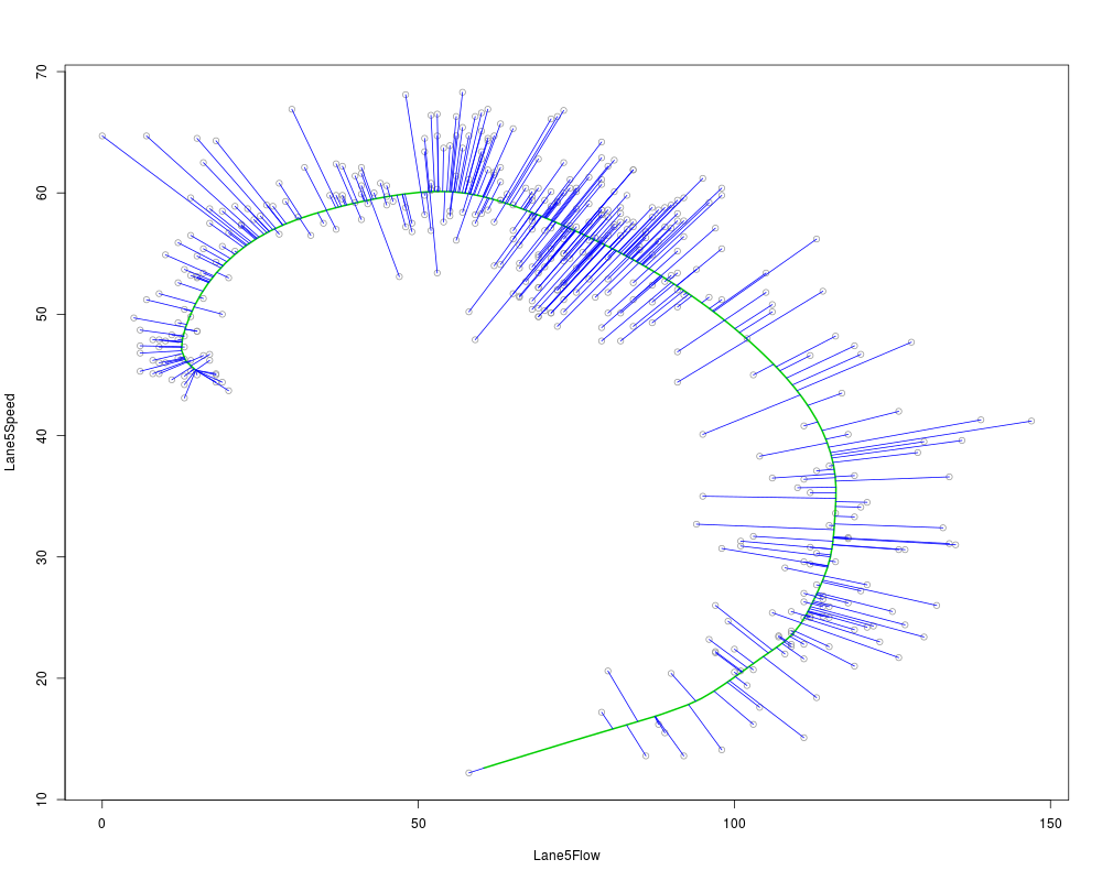
data(calspeedflow)
lpc1 <- lpc(calspeedflow[,3:4])
plot(lpc1, type=c("spline","project"), lwd=2)

Results


R version 3.3.1 (2016-06-21) -- "Bug in Your Hair"
Copyright (C) 2016 The R Foundation for Statistical Computing
Platform: x86_64-pc-linux-gnu (64-bit)

R is free software and comes with ABSOLUTELY NO WARRANTY.
You are welcome to redistribute it under certain conditions.
Type 'license()' or 'licence()' for distribution details.

R is a collaborative project with many contributors.
Type 'contributors()' for more information and
'citation()' on how to cite R or R packages in publications.

Type 'demo()' for some demos, 'help()' for on-line help, or
'help.start()' for an HTML browser interface to help.
Type 'q()' to quit R.

> library(LPCM)
> png(filename="/home/ddbj/snapshot/RGM3/R_CC/result/LPCM/plot.lpc.Rd_%03d_medium.png", width=480, height=480)
> ### Name: plot.lpc
> ### Title: Plotting local principal curves
> ### Aliases: plot.lpc plot.lpc.spline
> ### Keywords: multivariate
> 
> ### ** Examples
> 
> data(calspeedflow)
> lpc1 <- lpc(calspeedflow[,3:4])
> plot(lpc1, type=c("spline","project"), lwd=2)
> 
> 
> 
> 
> 
> dev.off()
null device 
          1 
>