LSTS Package

Description

This package has a set of functions that allows stationary analysis and locally stationary time series analysis.

Details

Acknowledgment

The first author gratefully acknowledges the financial support from Fondecyt grant 11121128.

Author(s)

Ricardo Olea <raolea@uc.cl>, Wilfredo Palma <wilfredo@mat.puc.cl>, Pilar Rubio <parubio@uc.cl>

Maintainer: Ricardo Olea <raolea@uc.cl>

References

Brockwell, Peter J., and Richard A. Davis. Introduction to time series and forecasting. 2002. ISBN-13: 978-0387953519.

Dahlhaus, R. Fitting time series models to nonstationary processes. The Annals of Statistics. 1997; Vol. 25, No. 1:1-37.

Dahlhaus, R. and Giraitis, L. On the optimal segment length for parameter estimates for locally stationary time series. Journal of Time Series Analysis. 1998; 19(6):629-655.

Palma W. Long-Memory Time Series. Theory and Methods. 1st ed. New Jersey: John Wiley & Sons, Inc.; 2007. 285 p.

Olea R, Palma W. An efficient estimator for locally stationary gaussian long-memory processes. The Annals of Statistics. 2010; Vol. 38, No. 5:2958-2997.

Palma W, Olea R, & Ferreira G. Estimation and forecasting of locally stationary processes. Journal of Forecasting. 2013; Vol. 32, No. 1:86-96.

Examples

##########################################
########## Tree Ring Aplication ##########
##########################################

## Require: "rdatamarket"
library(rdatamarket)
malleco = dmlist("22tn")

y = malleco$Value
op = par(mfrow = c(1,2), cex = 0.9)
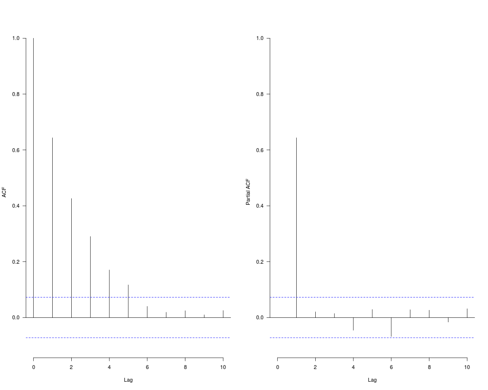
acf(y, lag = 10, ylim = c(-0.1,1), bty = "n", las = 1, main = "")
pacf(y, lag = 10, xlim = c(0,10), ylim = c(-0.1,1), bty = "n", las = 1, main = "")
par(op)
## AR(1) structure

y1 = y[1:250]
y2 = y[243:492]
y3 = y[485:734]
op = par(mfrow = c(2,3), cex = 0.9)
acf(y1, lag = 10, ylim = c(-0.1,1), bty = "n", las = 1, main = "block 1")
acf(y2, lag = 10, ylim = c(-0.1,1), bty = "n", las = 1, main = "block 2")
acf(y3, lag = 10, ylim = c(-0.1,1), bty = "n", las = 1, main = "block 3")
pacf(y1, lag = 10, xlim = c(0,10), ylim = c(-0.1,1), bty = "n", las = 1, main = "")
pacf(y2, lag = 10, xlim = c(0,10), ylim = c(-0.1,1), bty = "n", las = 1, main = "")
pacf(y3, lag = 10, xlim = c(0,10), ylim = c(-0.1,1), bty = "n", las = 1, main = "")
par(op)

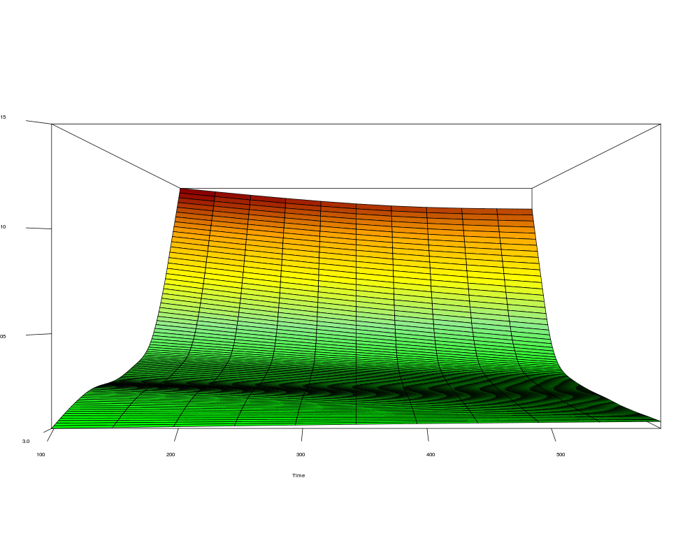
block.smooth.periodogram(y, spar.freq = 0.8, spar.time = 0.8, theta = 90, phi = 0)

# Analysis by blocks of phi and sigma parameters
T. = length(y)
N = 200
S = 100
M = trunc((T. - N)/S + 1)
table = c()
for(j in 1:M){
x = y[(1 + S*(j-1)):(N + S*(j-1))]
table = rbind(table,nlminb(start = c(0.65, 0.15), N = N, objective = LS.whittle.loglik,
                           series = x, order = c(p = 1, q = 0))$par)
}
u = (N/2 + S*(1:M-1))/T.
table = as.data.frame(cbind(u, table))
colnames(table) = c("u", "phi", "sigma")

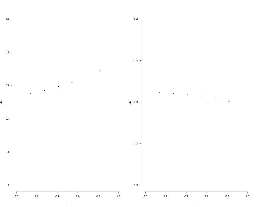
op = par(mfrow = c(1,2), cex = 0.8)
spar = 0.6
plot(smooth.spline(phi, spar = spar)$y ~ u, data = table, pch = 20, ylim = c(0,1),
     xlim = c(0,1), las = 1, bty = "n", ylab = expression(phi(u)))
plot(smooth.spline(sigma, spar = spar)$y ~ u, data = table, pch = 20, ylim = c(0,0.2),
     xlim = c(0,1), las = 1, bty = "n", ylab = expression(phi(u)))
par(op)

## start parameters
phi = smooth.spline(table$phi, spar = spar)$y
fit.1 = nls(phi ~ a0+a1*u, start = list(a0 = 0.65, a1 = 0.00))
sigma = smooth.spline(table$sigma, spar = spar)$y
fit.2 = nls(sigma ~ b0+b1*u, start = list(b0 = 0.65, b1 = 0.00))

fit = LS.whittle(series = y, start = c(coef(fit.1), coef(fit.2)), order = c(p = 1, q = 0),
                 ar.order = c(1), sd.order = 1, N = 180, n.ahead = 10)

## Summary
LS.summary(fit)

## Diagnostic
ts.diag(fit$residuals)

## Fitted Values
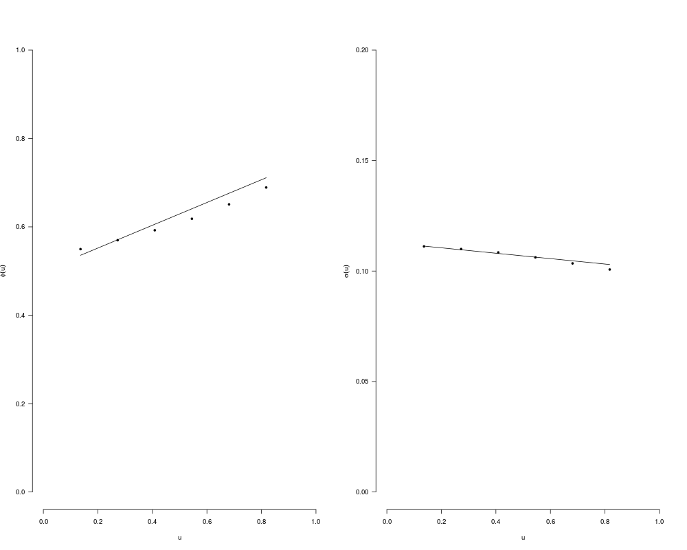
op = par(mfrow = c(1,2), cex = 0.8)
spar = 0.6
plot(smooth.spline(phi, spar = spar)$y ~ u, data = table, pch = 20, ylim = c(0,1),
     xlim = c(0,1), las = 1, bty = "n", ylab = expression(phi(u)))
lines(fit$coef[1]+fit$coef[2]*u~u)
plot(smooth.spline(sigma, spar = spar)$y ~ u, data = table, pch = 20, ylim = c(0,0.2),
     xlim = c(0,1), las = 1, bty = "n", ylab = expression(sigma(u)))
lines(fit$coef[3]+fit$coef[4]*u~u)
par(op)

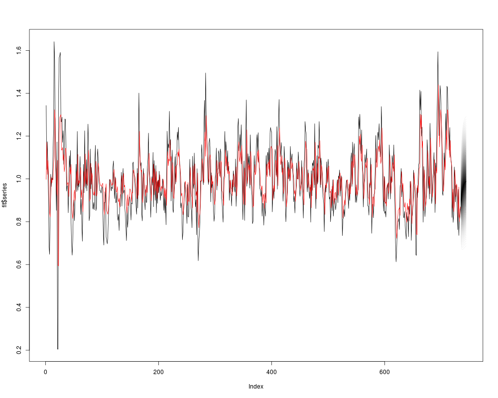
plot(fit$series, type = "l")
lines(fit$fitted.values, col = "red", lty = 1)
for(alpha in seq(0.05,1.00, 0.01)){
lines(fit$pred + fit$se * qnorm(1-alpha/2), col = gray(1-alpha))
lines(fit$pred - fit$se * qnorm(1-alpha/2), col = gray(1-alpha))
}

Results

R version 3.3.1 (2016-06-21) -- "Bug in Your Hair"
Copyright (C) 2016 The R Foundation for Statistical Computing
Platform: x86_64-pc-linux-gnu (64-bit)

R is free software and comes with ABSOLUTELY NO WARRANTY.
You are welcome to redistribute it under certain conditions.
Type 'license()' or 'licence()' for distribution details.

R is a collaborative project with many contributors.
Type 'contributors()' for more information and
'citation()' on how to cite R or R packages in publications.

Type 'demo()' for some demos, 'help()' for on-line help, or
'help.start()' for an HTML browser interface to help.
Type 'q()' to quit R.

> library(LSTS)
> png(filename="/home/ddbj/snapshot/RGM3/R_CC/result/LSTS/LSTS-package.Rd_%03d_medium.png", width=480, height=480)
> ### Name: LSTS-package
> ### Title: LSTS Package
> ### Aliases: LSTS-package LSTS
> ### Keywords: package
> 
> ### ** Examples
> 
> ##########################################
> ########## Tree Ring Aplication ##########
> ##########################################
> 
> ## Require: "rdatamarket"
> library(rdatamarket)
Loading required package: zoo

Attaching package: 'zoo'

The following objects are masked from 'package:base':

    as.Date, as.Date.numeric

> malleco = dmlist("22tn")
> 
> y = malleco$Value
> op = par(mfrow = c(1,2), cex = 0.9)
> acf(y, lag = 10, ylim = c(-0.1,1), bty = "n", las = 1, main = "")
> pacf(y, lag = 10, xlim = c(0,10), ylim = c(-0.1,1), bty = "n", las = 1, main = "")
> par(op)
> ## AR(1) structure
> 
> y1 = y[1:250]
> y2 = y[243:492]
> y3 = y[485:734]
> op = par(mfrow = c(2,3), cex = 0.9)
> acf(y1, lag = 10, ylim = c(-0.1,1), bty = "n", las = 1, main = "block 1")
> acf(y2, lag = 10, ylim = c(-0.1,1), bty = "n", las = 1, main = "block 2")
> acf(y3, lag = 10, ylim = c(-0.1,1), bty = "n", las = 1, main = "block 3")
> pacf(y1, lag = 10, xlim = c(0,10), ylim = c(-0.1,1), bty = "n", las = 1, main = "")
> pacf(y2, lag = 10, xlim = c(0,10), ylim = c(-0.1,1), bty = "n", las = 1, main = "")
> pacf(y3, lag = 10, xlim = c(0,10), ylim = c(-0.1,1), bty = "n", las = 1, main = "")
> par(op)
> 
> block.smooth.periodogram(y, spar.freq = 0.8, spar.time = 0.8, theta = 90, phi = 0)
> 
> # Analysis by blocks of phi and sigma parameters
> T. = length(y)
> N = 200
> S = 100
> M = trunc((T. - N)/S + 1)
> table = c()
> for(j in 1:M){
+ x = y[(1 + S*(j-1)):(N + S*(j-1))]
+ table = rbind(table,nlminb(start = c(0.65, 0.15), N = N, objective = LS.whittle.loglik,
+                            series = x, order = c(p = 1, q = 0))$par)
+ }
> u = (N/2 + S*(1:M-1))/T.
> table = as.data.frame(cbind(u, table))
> colnames(table) = c("u", "phi", "sigma")
> 
> op = par(mfrow = c(1,2), cex = 0.8)
> spar = 0.6
> plot(smooth.spline(phi, spar = spar)$y ~ u, data = table, pch = 20, ylim = c(0,1),
+      xlim = c(0,1), las = 1, bty = "n", ylab = expression(phi(u)))
> plot(smooth.spline(sigma, spar = spar)$y ~ u, data = table, pch = 20, ylim = c(0,0.2),
+      xlim = c(0,1), las = 1, bty = "n", ylab = expression(phi(u)))
> par(op)
> 
> ## start parameters
> phi = smooth.spline(table$phi, spar = spar)$y
> fit.1 = nls(phi ~ a0+a1*u, start = list(a0 = 0.65, a1 = 0.00))
> sigma = smooth.spline(table$sigma, spar = spar)$y
> fit.2 = nls(sigma ~ b0+b1*u, start = list(b0 = 0.65, b1 = 0.00))
> 
> fit = LS.whittle(series = y, start = c(coef(fit.1), coef(fit.2)), order = c(p = 1, q = 0),
+                  ar.order = c(1), sd.order = 1, N = 180, n.ahead = 10)
> 
> ## Summary
> LS.summary(fit)
$summary
   Estimate Std. Error z-value Pr(>|z|)
a0   0.5006     0.0709  7.0605   0.0000
a1   0.2577     0.1263  2.0409   0.0413
b0   0.1130     0.0028 40.7288   0.0000
b1  -0.0122     0.0051 -2.3845   0.0171

$aic
[1] -5.313435

$npar
[1] 4

> 
> ## Diagnostic
> ts.diag(fit$residuals)
> 
> ## Fitted Values
> op = par(mfrow = c(1,2), cex = 0.8)
> spar = 0.6
> plot(smooth.spline(phi, spar = spar)$y ~ u, data = table, pch = 20, ylim = c(0,1),
+      xlim = c(0,1), las = 1, bty = "n", ylab = expression(phi(u)))
> lines(fit$coef[1]+fit$coef[2]*u~u)
> plot(smooth.spline(sigma, spar = spar)$y ~ u, data = table, pch = 20, ylim = c(0,0.2),
+      xlim = c(0,1), las = 1, bty = "n", ylab = expression(sigma(u)))
> lines(fit$coef[3]+fit$coef[4]*u~u)
> par(op)
> 
> plot(fit$series, type = "l")
> lines(fit$fitted.values, col = "red", lty = 1)
> for(alpha in seq(0.05,1.00, 0.01)){
+ lines(fit$pred + fit$se * qnorm(1-alpha/2), col = gray(1-alpha))
+ lines(fit$pred - fit$se * qnorm(1-alpha/2), col = gray(1-alpha))
+ }
> 
> 
> 
> 
> 
> dev.off()
null device 
          1 
>