R Graphical Manual

Browse All

Last data update: 2014.03.03

R: Smooth Periodogram by blocks

block.smooth.periodogram

R Documentation

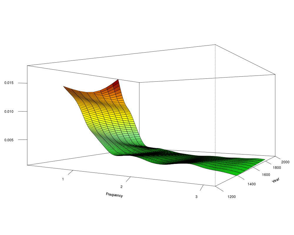
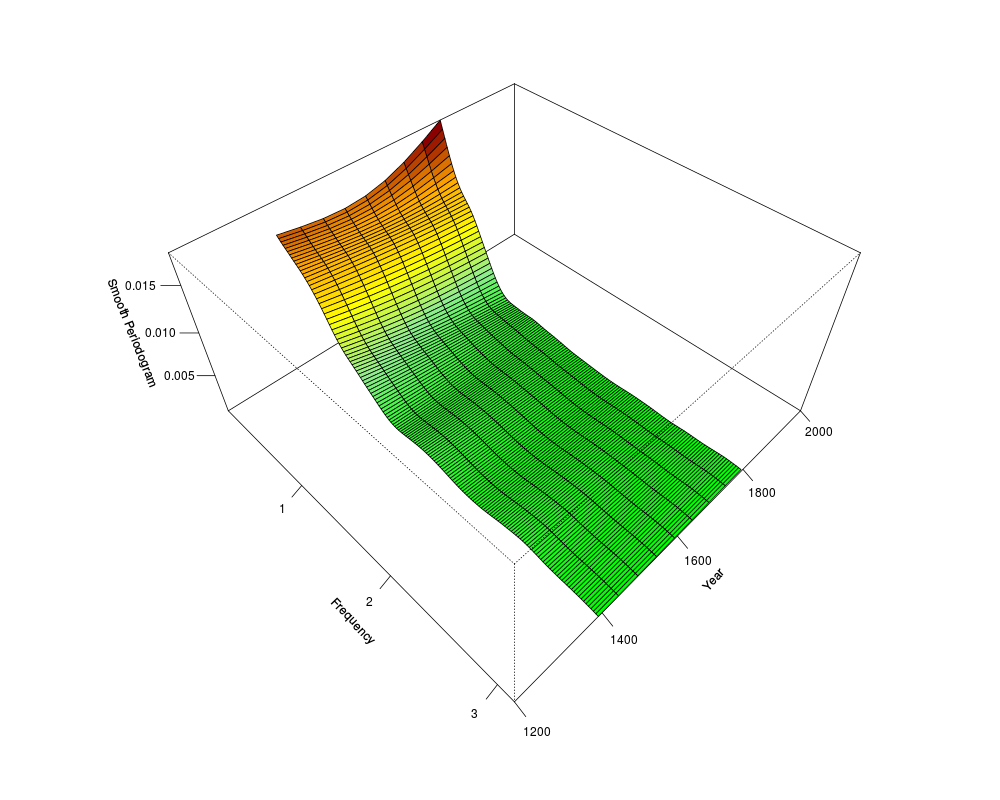
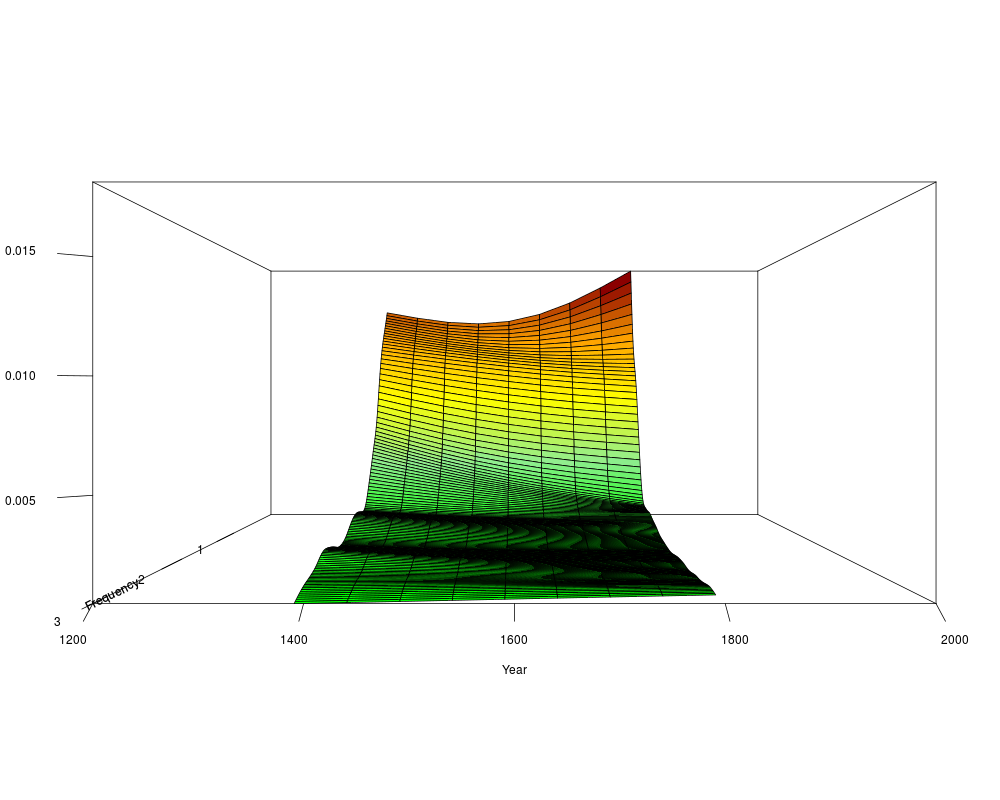
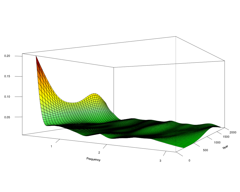
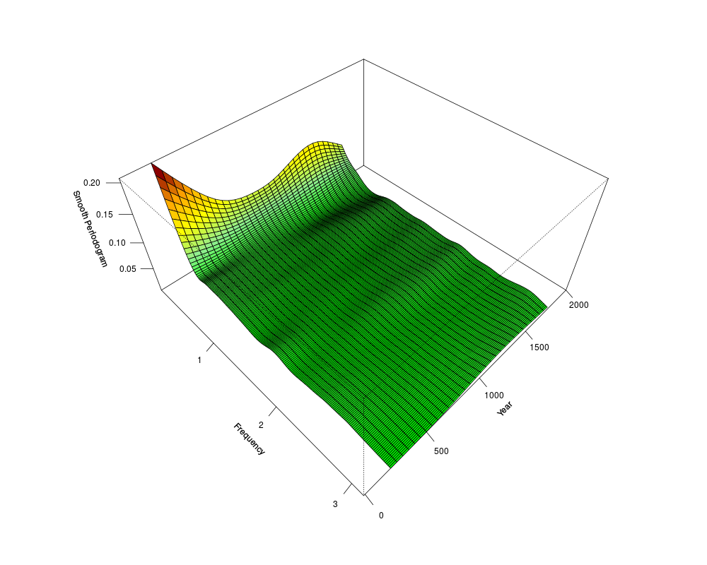
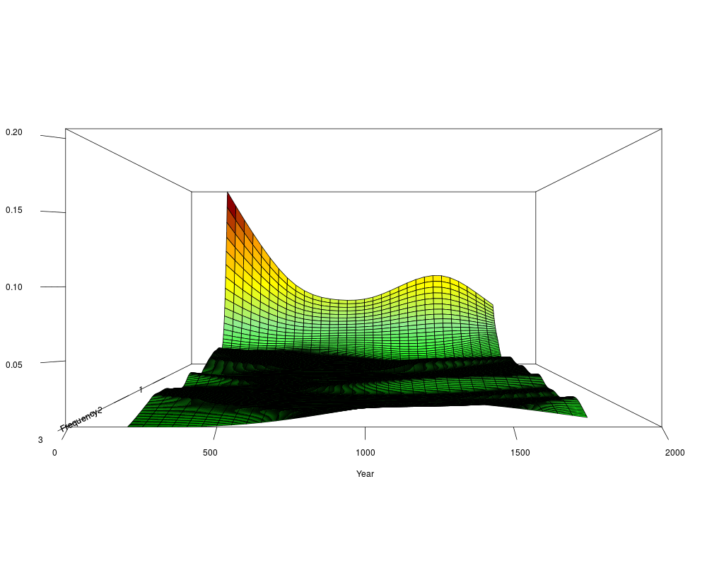
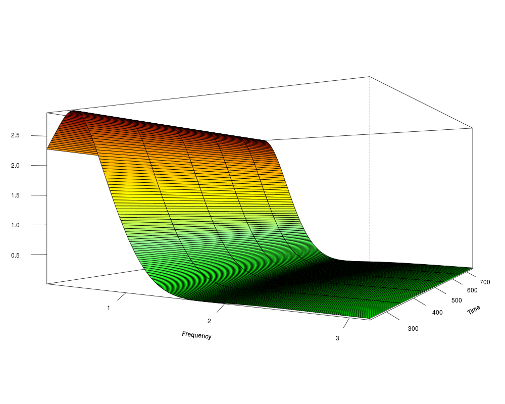
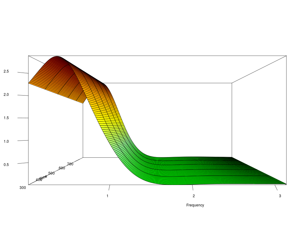
Smooth Periodogram by blocks

Description

Plot in 3D the smoothing periodogram of a time series, by blocks or windows.

Usage

block.smooth.periodogram(y, x = NULL, N = NULL, S = NULL, p = 0.25,
                         spar.freq = 0, spar.time = 0, theta = 0, phi = 0,
                         xlim = NULL, ylim = NULL, zlim = NULL, ylab = "Time",
                         palette.col = NULL)

Arguments

`y`	data vector.
`x`	optional vector, if `x=NULL` then the function uses `x=1:n` where `n` is the length of `y`. More details in '`y`' argument from `persp` function.
`N`	value corresponding to the length of the window to compute periodogram. If `N=NULL` then the function will use N = \textmd{trunc}(n^{0.8}), see Dahlhaus (1998) where n is the length of the `y` vector.
`S`	value corresponding to the lag with which will be taking the blocks or windows to calculate the periodogram.
`p`	value used if it is desired that `S` is proportional to `N`. By default `p=0.25`, if `S` and `N` are not entered.
`spar.freq, spar.time`	smoothing parameter, typically (but not necessarily) in (0,1].
`theta, phi`	angles defining the viewing direction. `theta` gives the azimuthal direction and `phi` the colatitude.
`xlim, ylim, zlim`	x-,y- and z-limits. They are `NULL` by default and they are optionals parameters.
`ylab`	title for 'y' axis. Optional argument, by default is `ylab="Time"`. This must be character strings.
`palette.col`	colors palette.

Details

The number of windows of the function is M = \textmd{trunc}((n-N)/S+1), where trunc truncates de entered value and n is the length of the vector y. All windows are of the same length N, if this value isn't entered by user then is computed as N=\textmd{trunc}(n^{0.8}) (Dahlhaus).

block.smooth.periodogram computes the periodogram in each of the M windows and then smoothes it two times with smooth.spline function; the first time using spar.freq parameter and the second time with spar.time. These windows overlap between them.

The surface is then viewed by looking at the origin from a direction defined by theta and phi. If theta and phi are both zero the viewing direction is directly down the negative y axis. Changing theta will vary the azimuth and changing phi the colatitude.

Author(s)

Ricardo Olea <raolea@uc.cl>

References

Dahlhaus, R. Fitting time series models to nonstationary processes. The Annals of Statistics. 1997; Vol. 25, No. 1:1-37.

Dahlhaus, R. and Giraitis, L. On the optimal segment length for parameter estimates for locally stationary time series. Journal of Time Series Analysis. 1998; 19(6):629-655.

Examples

## Require "rdatamarket"
library(rdatamarket)

malleco = dmlist("22tn")
mammothcreek = dmlist("22r7")


## Example 1
block.smooth.periodogram(y = malleco$Value, x = malleco$Year, spar.freq = .7,
                         spar.time = .7, theta = 30, phi =  0, N = 300, S = 50, 
                         ylim = c(1200,2000), ylab = "Year")
block.smooth.periodogram(y = malleco$Value, x = malleco$Year, spar.freq = .7, 
                         spar.time = .7, theta = 45, phi = 45, N = 300, S = 50,
                         ylim = c(1200,2000), ylab = "Year")
block.smooth.periodogram(y = malleco$Value, x = malleco$Year, spar.freq = .7, 
                         spar.time = .7, theta = 90, phi =  0, N = 300, S = 50,
                         ylim = c(1200,2000), ylab = "Year")

## Example 2
block.smooth.periodogram(y = mammothcreek$Value, x = mammothcreek$Year, spar.freq = .7,
                         spar.time = .7, theta = 30, phi =  0, N = 400, S = 50,
                         ylim = c(-10,2000), ylab = "Year")
block.smooth.periodogram(y = mammothcreek$Value, x = mammothcreek$Year, spar.freq = .7,
                         spar.time = .7, theta = 45, phi = 45, N = 400, S = 50, 
                         ylim = c(-10,2000), ylab = "Year")
block.smooth.periodogram(y = mammothcreek$Value, x = mammothcreek$Year, spar.freq = .7, 
                         spar.time = .7, theta = 90, phi = 0, N = 400, S = 50, 
                         ylim = c(-10,2000), ylab = "Year")

## Example 3: Simulated AR(2)
set.seed(2015)
ts.sim = arima.sim(n = 1000, model = list(order = c(2,0,0), ar = c(1.3, -0.6)))
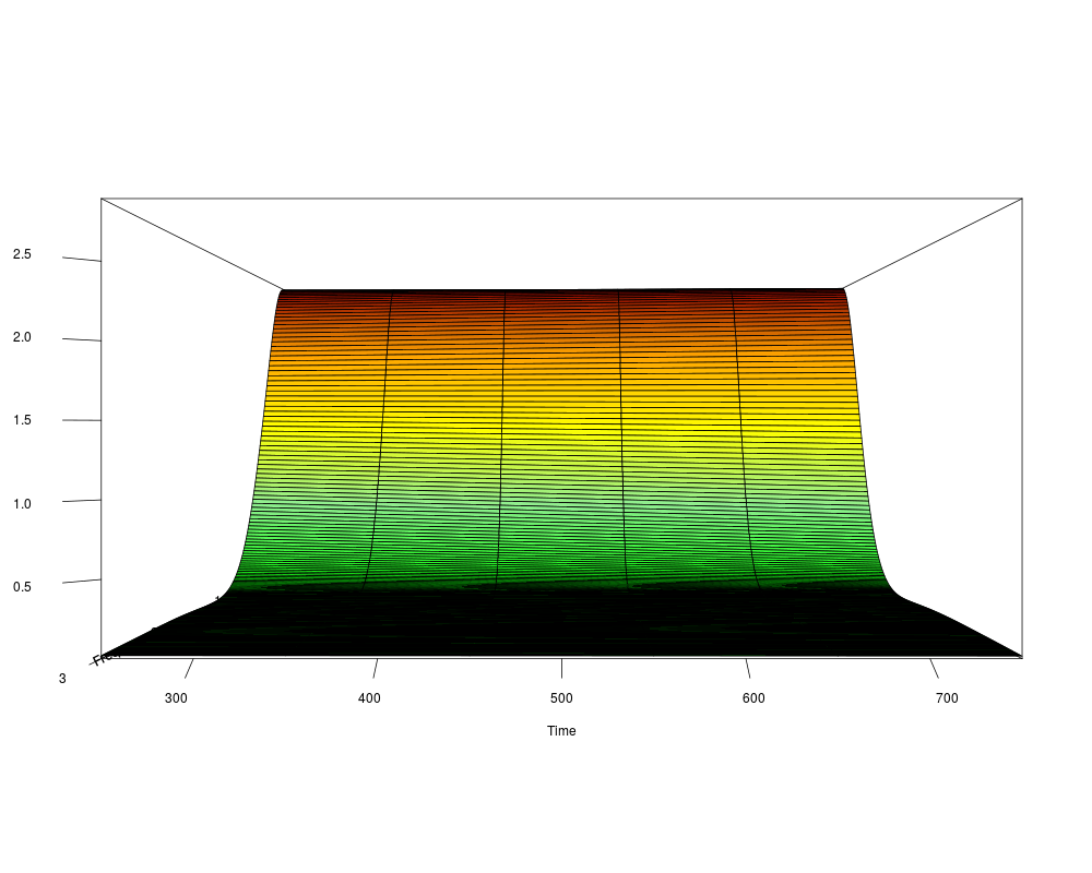
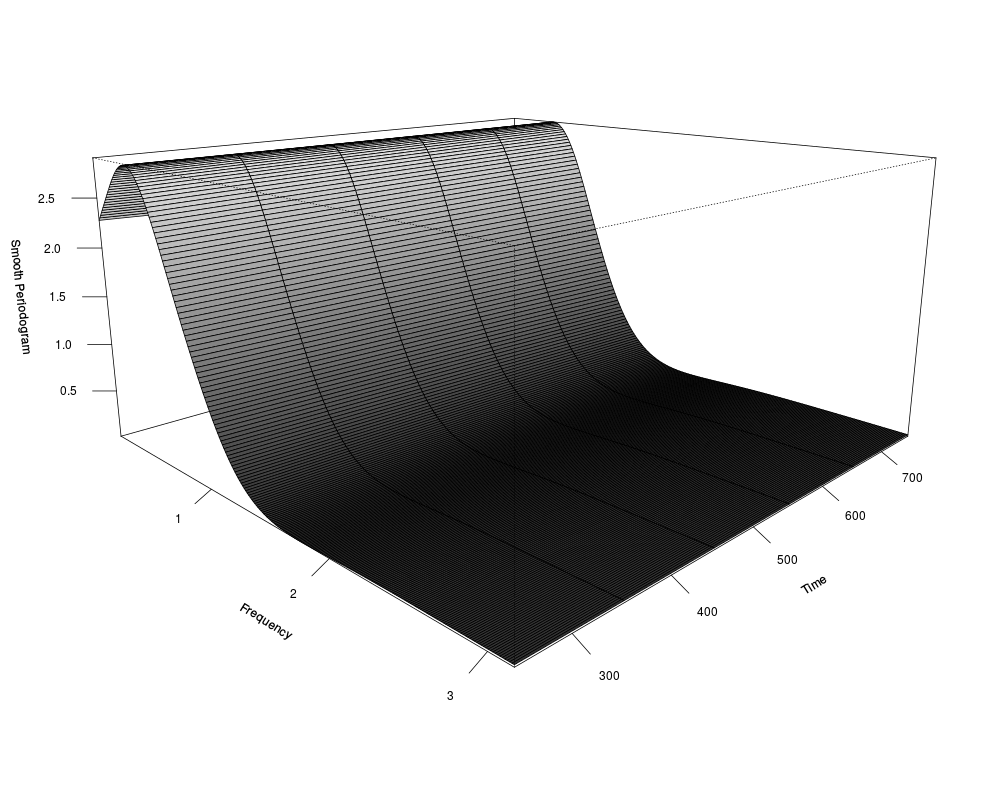
block.smooth.periodogram(y = ts.sim, spar.freq = .9, spar.time = .9, theta = 30, phi = 00, 
                         N = 500, S = 100, ylab = "Time")
block.smooth.periodogram(y = ts.sim, spar.freq = .9, spar.time = .9, theta = 00, phi = 00, 
                         N = 500, S = 100, ylab = "Time")
block.smooth.periodogram(y = ts.sim, spar.freq = .9, spar.time = .9, theta = 90, phi = 00,
                         N = 500, S = 100, ylab = "Time")
block.smooth.periodogram(y = ts.sim, spar.freq = .9, spar.time = .9, theta = 45, phi = 15, 
                         N = 500, S = 100, ylab = "Time")
block.smooth.periodogram(y = ts.sim, spar.freq = .9, spar.time = .9, theta = 45, phi = 15, 
                         N = 500, S = 100, ylab = "Time", 
                         palette.col = gray(level = seq(0.2,0.9,0.1 )))

Results


R version 3.3.1 (2016-06-21) -- "Bug in Your Hair"
Copyright (C) 2016 The R Foundation for Statistical Computing
Platform: x86_64-pc-linux-gnu (64-bit)

R is free software and comes with ABSOLUTELY NO WARRANTY.
You are welcome to redistribute it under certain conditions.
Type 'license()' or 'licence()' for distribution details.

R is a collaborative project with many contributors.
Type 'contributors()' for more information and
'citation()' on how to cite R or R packages in publications.

Type 'demo()' for some demos, 'help()' for on-line help, or
'help.start()' for an HTML browser interface to help.
Type 'q()' to quit R.

> library(LSTS)
> png(filename="/home/ddbj/snapshot/RGM3/R_CC/result/LSTS/block.smooth.periodogram.Rd_%03d_medium.png", width=480, height=480)
> ### Name: block.smooth.periodogram
> ### Title: Smooth Periodogram by blocks
> ### Aliases: block.smooth.periodogram
> ### Keywords: Fourier smooth timeseries
> 
> ### ** Examples
> 
> ## Require "rdatamarket"
> library(rdatamarket)
Loading required package: zoo

Attaching package: 'zoo'

The following objects are masked from 'package:base':

    as.Date, as.Date.numeric

> 
> malleco = dmlist("22tn")
> mammothcreek = dmlist("22r7")
> 
> 
> ## Example 1
> block.smooth.periodogram(y = malleco$Value, x = malleco$Year, spar.freq = .7,
+                          spar.time = .7, theta = 30, phi =  0, N = 300, S = 50, 
+                          ylim = c(1200,2000), ylab = "Year")
> block.smooth.periodogram(y = malleco$Value, x = malleco$Year, spar.freq = .7, 
+                          spar.time = .7, theta = 45, phi = 45, N = 300, S = 50,
+                          ylim = c(1200,2000), ylab = "Year")
> block.smooth.periodogram(y = malleco$Value, x = malleco$Year, spar.freq = .7, 
+                          spar.time = .7, theta = 90, phi =  0, N = 300, S = 50,
+                          ylim = c(1200,2000), ylab = "Year")
> 
> ## Example 2
> block.smooth.periodogram(y = mammothcreek$Value, x = mammothcreek$Year, spar.freq = .7,
+                          spar.time = .7, theta = 30, phi =  0, N = 400, S = 50,
+                          ylim = c(-10,2000), ylab = "Year")
> block.smooth.periodogram(y = mammothcreek$Value, x = mammothcreek$Year, spar.freq = .7,
+                          spar.time = .7, theta = 45, phi = 45, N = 400, S = 50, 
+                          ylim = c(-10,2000), ylab = "Year")
> block.smooth.periodogram(y = mammothcreek$Value, x = mammothcreek$Year, spar.freq = .7, 
+                          spar.time = .7, theta = 90, phi = 0, N = 400, S = 50, 
+                          ylim = c(-10,2000), ylab = "Year")
> 
> ## Example 3: Simulated AR(2)
> set.seed(2015)
> ts.sim = arima.sim(n = 1000, model = list(order = c(2,0,0), ar = c(1.3, -0.6)))
> block.smooth.periodogram(y = ts.sim, spar.freq = .9, spar.time = .9, theta = 30, phi = 00, 
+                          N = 500, S = 100, ylab = "Time")
> block.smooth.periodogram(y = ts.sim, spar.freq = .9, spar.time = .9, theta = 00, phi = 00, 
+                          N = 500, S = 100, ylab = "Time")
> block.smooth.periodogram(y = ts.sim, spar.freq = .9, spar.time = .9, theta = 90, phi = 00,
+                          N = 500, S = 100, ylab = "Time")
> block.smooth.periodogram(y = ts.sim, spar.freq = .9, spar.time = .9, theta = 45, phi = 15, 
+                          N = 500, S = 100, ylab = "Time")
> block.smooth.periodogram(y = ts.sim, spar.freq = .9, spar.time = .9, theta = 45, phi = 15, 
+                          N = 500, S = 100, ylab = "Time", 
+                          palette.col = gray(level = seq(0.2,0.9,0.1 )))
> 
> 
> 
> 
> 
> dev.off()
null device 
          1 
>