Fit a conditional inference survival tree for LTRC data

Description

LTRCIT returns an party object. This function extends the conditional inference survival tree algorithm in ctree to fit left-truncated and right censored (LTRC) data.

Usage

LTRCIT(Formula, Data, Control = partykit::ctree_control())

Arguments

Value

An object of class party.

References

Fu, W. and Simonoff, J.S.(2016). Survival trees for left-truncated and right-censored data, with application to time-varying covariate data. arXiv:1606.03033 [stat.ME]

Examples

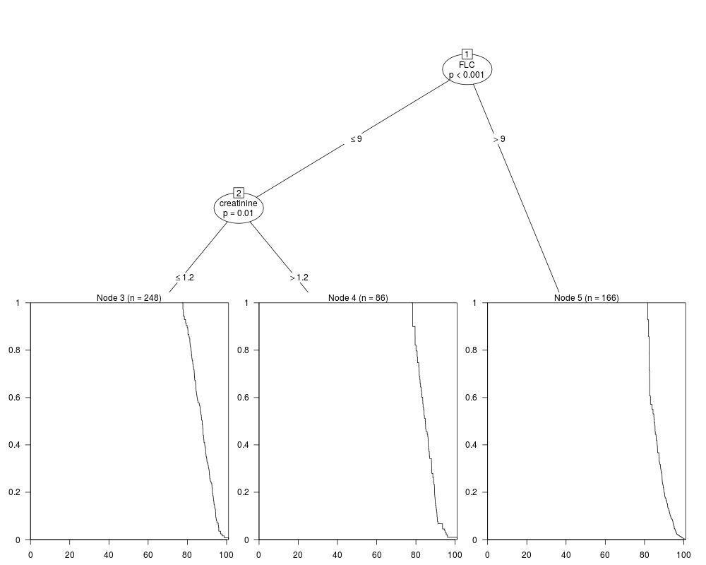
## The Assay of serum free light chain data in survival package
## Adjust data & clean data
library(survival)
library(LTRCtrees)
Data <- flchain
Data <- Data[!is.na(Data$creatinine),]
Data$End <- Data$age + Data$futime/365
DATA <- Data[Data$End > Data$age,]
names(DATA)[6] <- "FLC"

## Setup training set and test set
Train = DATA[1:500,]
Test = DATA[1000:1020,]

## Fit LTRCIT survival tree
LTRCIT.obj <-  LTRCIT(Surv(age, End, death) ~ sex + FLC + creatinine, Train)
plot(LTRCIT.obj)

## Putting Surv(End, death) in formula would result an error message
## since LTRCIT is expecting Surv(time1, time2, event)

## Note that LTRCIT.obj is an object of class party
## predict median survival time on test data
LTRCIT.pred <- predict(LTRCIT.obj, newdata = Test, type = "response")

## predict Kaplan Meier survival curve on test data,
## return a list of survfit objects -- the predicted KM curves
LTRCIT.pred <- predict(LTRCIT.obj, newdata = Test, type = "prob")

####################################################################
####### Survival tree with time-varying covariates ##################
####################################################################
## The pbcseq dataset of survival package
library(survival)
## Create the start-stop-event triplet needed for coxph and LTRC trees
first <- with(pbcseq, c(TRUE, diff(id) !=0)) #first id for each subject
last <- c(first[-1], TRUE) #last id
time1 <- with(pbcseq, ifelse(first, 0, day))
time2 <- with(pbcseq, ifelse(last, futime, c(day[-1], 0)))
event <- with(pbcseq, ifelse(last, status, 0))
event <- 1*(event==2)

pbcseq$time1 <- time1
pbcseq$time2 <- time2
pbcseq$event <-  event

pbcseq = pbcseq[1:1000,] ## fit on subset of the data to save fitting time
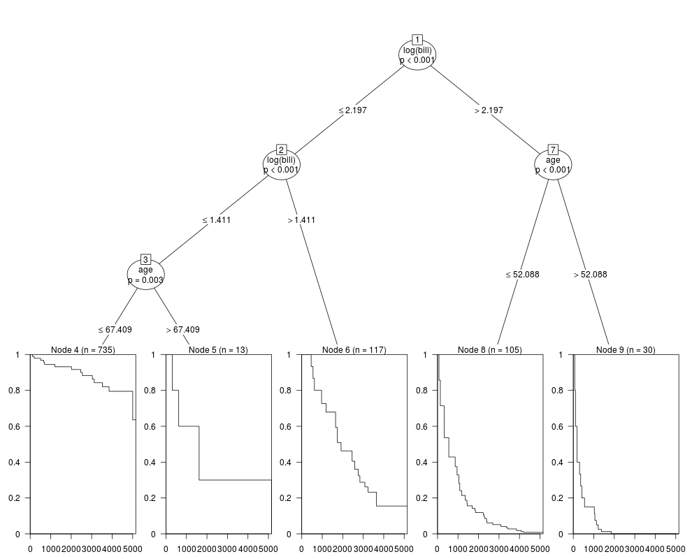
## Fit the Cox model and LTRCIT tree with time-varying covariates
fit.cox <- coxph(Surv(time1, time2, event) ~ age + sex + log(bili), pbcseq)
LTRCIT.fit <- LTRCIT(Surv(time1, time2, event) ~ age + sex + log(bili), pbcseq)
plot(LTRCIT.fit)

## transform the wide format data into long format data using tmerge function
## from survival function
## Stanford Heart Transplant data
jasa$subject <- 1:nrow(jasa)

tdata <- with(jasa, data.frame(subject = subject,
                              futime= pmax(.5, fu.date - accept.dt),
                              txtime= ifelse(tx.date== fu.date,
                                             (tx.date -accept.dt) -.5,
                                             (tx.date - accept.dt)),
                              fustat = fustat))

sdata <- tmerge(jasa, tdata, id=subject,death = event(futime, fustat),
                   trt = tdc(txtime), options= list(idname="subject"))

sdata$age <- sdata$age - 48

sdata$year <- as.numeric(sdata$accept.dt - as.Date("1967-10-01"))/365.25

Cox.fit <- coxph(Surv(tstart, tstop, death) ~ age+ surgery, data= sdata)
LTRCART.fit <- LTRCART(Surv(tstart, tstop, death) ~ age + transplant, data = sdata)
plot(LTRCIT.fit)

Results

R version 3.3.1 (2016-06-21) -- "Bug in Your Hair"
Copyright (C) 2016 The R Foundation for Statistical Computing
Platform: x86_64-pc-linux-gnu (64-bit)

R is free software and comes with ABSOLUTELY NO WARRANTY.
You are welcome to redistribute it under certain conditions.
Type 'license()' or 'licence()' for distribution details.

R is a collaborative project with many contributors.
Type 'contributors()' for more information and
'citation()' on how to cite R or R packages in publications.

Type 'demo()' for some demos, 'help()' for on-line help, or
'help.start()' for an HTML browser interface to help.
Type 'q()' to quit R.

> library(LTRCtrees)
> png(filename="/home/ddbj/snapshot/RGM3/R_CC/result/LTRCtrees/LTRCIT.Rd_%03d_medium.png", width=480, height=480)
> ### Name: LTRCIT
> ### Title: Fit a conditional inference survival tree for LTRC data
> ### Aliases: LTRCIT
> 
> ### ** Examples
> 
> ## The Assay of serum free light chain data in survival package
> ## Adjust data & clean data
> library(survival)
> library(LTRCtrees)
> Data <- flchain
> Data <- Data[!is.na(Data$creatinine),]
> Data$End <- Data$age + Data$futime/365
> DATA <- Data[Data$End > Data$age,]
> names(DATA)[6] <- "FLC"
> 
> ## Setup training set and test set
> Train = DATA[1:500,]
> Test = DATA[1000:1020,]
> 
> ## Fit LTRCIT survival tree
> LTRCIT.obj <-  LTRCIT(Surv(age, End, death) ~ sex + FLC + creatinine, Train)
> plot(LTRCIT.obj)
> 
> ## Putting Surv(End, death) in formula would result an error message
> ## since LTRCIT is expecting Surv(time1, time2, event)
> 
> ## Note that LTRCIT.obj is an object of class party
> ## predict median survival time on test data
> LTRCIT.pred <- predict(LTRCIT.obj, newdata = Test, type = "response")
> 
> ## predict Kaplan Meier survival curve on test data,
> ## return a list of survfit objects -- the predicted KM curves
> LTRCIT.pred <- predict(LTRCIT.obj, newdata = Test, type = "prob")
> 
> ####################################################################
> ####### Survival tree with time-varying covariates ##################
> ####################################################################
> ## The pbcseq dataset of survival package
> library(survival)
> ## Create the start-stop-event triplet needed for coxph and LTRC trees
> first <- with(pbcseq, c(TRUE, diff(id) !=0)) #first id for each subject
> last <- c(first[-1], TRUE) #last id
> time1 <- with(pbcseq, ifelse(first, 0, day))
> time2 <- with(pbcseq, ifelse(last, futime, c(day[-1], 0)))
> event <- with(pbcseq, ifelse(last, status, 0))
> event <- 1*(event==2)
> 
> pbcseq$time1 <- time1
> pbcseq$time2 <- time2
> pbcseq$event <-  event
> 
> pbcseq = pbcseq[1:1000,] ## fit on subset of the data to save fitting time
> ## Fit the Cox model and LTRCIT tree with time-varying covariates
> fit.cox <- coxph(Surv(time1, time2, event) ~ age + sex + log(bili), pbcseq)
> LTRCIT.fit <- LTRCIT(Surv(time1, time2, event) ~ age + sex + log(bili), pbcseq)
> plot(LTRCIT.fit)
> 
> ## transform the wide format data into long format data using tmerge function
> ## from survival function
> ## Stanford Heart Transplant data
> jasa$subject <- 1:nrow(jasa)
> 
> tdata <- with(jasa, data.frame(subject = subject,
+                               futime= pmax(.5, fu.date - accept.dt),
+                               txtime= ifelse(tx.date== fu.date,
+                                              (tx.date -accept.dt) -.5,
+                                              (tx.date - accept.dt)),
+                               fustat = fustat))
> 
> sdata <- tmerge(jasa, tdata, id=subject,death = event(futime, fustat),
+                    trt = tdc(txtime), options= list(idname="subject"))
> 
> sdata$age <- sdata$age - 48
> 
> sdata$year <- as.numeric(sdata$accept.dt - as.Date("1967-10-01"))/365.25
> 
> Cox.fit <- coxph(Surv(tstart, tstop, death) ~ age+ surgery, data= sdata)
> LTRCART.fit <- LTRCART(Surv(tstart, tstop, death) ~ age + transplant, data = sdata)
> plot(LTRCIT.fit)
> 
> 
> 
> 
> 
> 
> dev.off()
null device 
          1 
>