Batting table

Description

Batting table - batting statistics

Usage

data(Batting)

Format

A data frame with 99846 observations on the following 22 variables.

playerID

Player ID code

yearID

Year

stint

player's stint (order of appearances within a season)

teamID

Team; a factor

lgID

League; a factor with levels AA AL FL NL PL UA

G

Games: number of games in which a player played

AB

At Bats

R

Runs

H

Hits: times reached base because of a batted, fair ball without error by the defense

X2B

Doubles: hits on which the batter reached second base safely

X3B

Triples: hits on which the batter reached third base safely

HR

Homeruns

RBI

Runs Batted In

SB

Stolen Bases

CS

Caught Stealing

BB

Base on Balls

SO

Strikeouts

IBB

Intentional walks

HBP

Hit by pitch

SH

Sacrifice hits

SF

Sacrifice flies

GIDP

Grounded into double plays

Details

Variables X2B and X3B are named 2B and 3B in the original database

Source

Lahman, S. (2015) Lahman's Baseball Database, 1871-2014, 2015 version, http://baseball1.com/statistics/

See Also

battingStats for calculating batting average (BA) and other derived statistics

baseball for a similar dataset, but a subset of players who played 15 or more seasons.

Baseball for data on batting in the 1987 season.

Examples

data(Batting)
head(Batting)
require('plyr')

# calculate batting average and other stats
batting <- battingStats()

# add salary to Batting data; need to match by player, year and team
batting <- merge(batting, 
                 Salaries[,c("playerID", "yearID", "teamID", "salary")], 
                 by=c("playerID", "yearID", "teamID"), all.x=TRUE)

# Add name, age and bat hand information:
masterInfo <- Master[, c('playerID', 'birthYear', 'birthMonth',
                          'nameLast', 'nameFirst', 'bats')]
batting <- merge(batting, masterInfo, all.x = TRUE)
batting$age <- with(batting, yearID - birthYear -
                             ifelse(birthMonth < 10, 0, 1))

batting <- arrange(batting, playerID, yearID, stint)

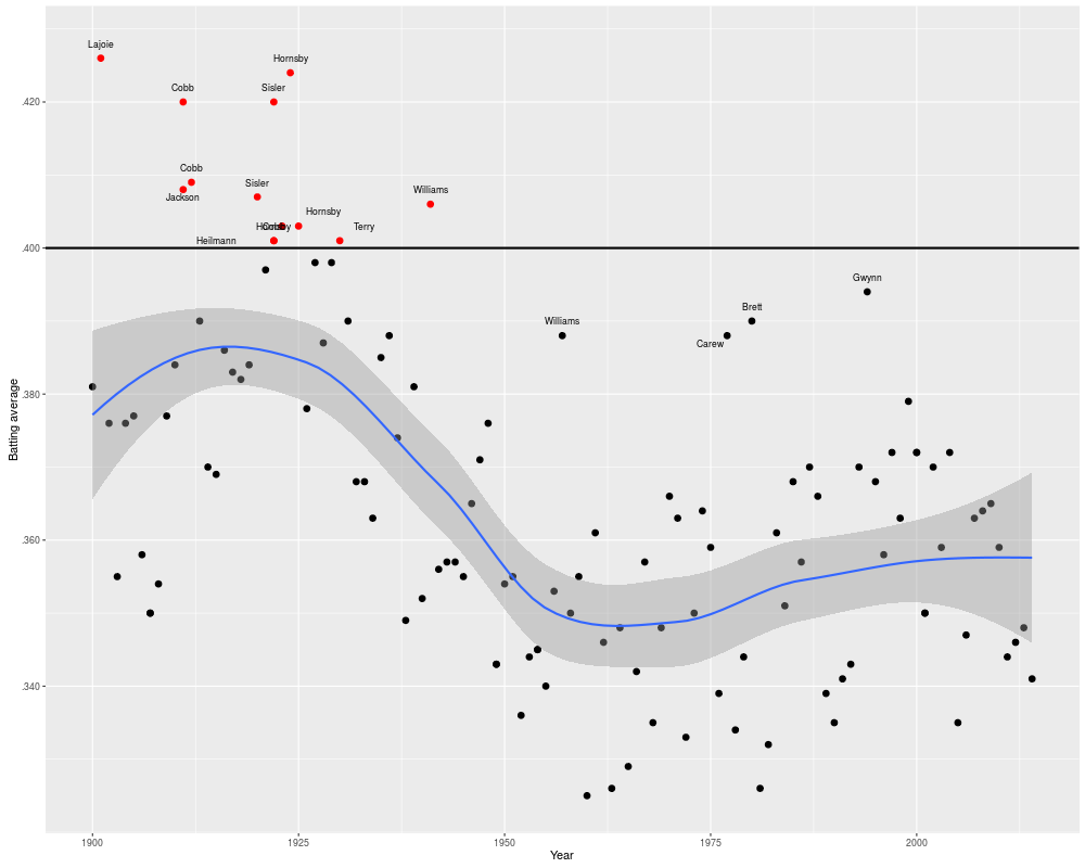
## Generate a ggplot similar to the NYT graph in the story about Ted
## Williams and the last .400 MLB season 
# http://www.nytimes.com/interactive/2011/09/18/sports/baseball/WILLIAMS-GRAPHIC.html

# Restrict the pool of eligible players to the years after 1899 and
# players with a minimum of 450 plate appearances (this covers the
# strike year of 1994 when Tony Gwynn hit .394 before play was suspended
# for the season - in a normal year, the minimum number of plate appearances is 502)
eligibleHitters <- subset(batting, yearID >= 1900 & PA > 450)

# Find the hitters with the highest BA in MLB each year (there are a
# few ties).  Include all players with BA > .400
topHitters <- ddply(eligibleHitters, .(yearID), subset, (BA == max(BA))|BA > .400)

# Create a factor variable to distinguish the .400 hitters
topHitters$ba400 <- with(topHitters, BA >= 0.400)

# Sub-data frame for the .400 hitters plus the outliers after 1950
# (averages above .380) - used to produce labels in the plot below
bignames <- rbind(subset(topHitters, ba400),
                  subset(topHitters, yearID > 1950 & BA > 0.380))
# Cut to the relevant set of variables
bignames <- subset(bignames, select = c('playerID', 'yearID', 'nameLast',
                                        'nameFirst', 'BA'))

# Ditto for the original data frame
topHitters <- subset(topHitters, select = c('playerID', 'yearID', 'BA', 'ba400'))

# Positional offsets to spread out certain labels
#                     NL TC JJ TC GS TC RH GS HH RH RH BT TW TW  RC GB TG 
bignames$xoffset <- c(0, 0, 0, 0, 0, 0, 0, 0, -8, 0, 3, 3, 0, 0, -2, 0, 0)
bignames$yoffset <- c(0, 0, -0.003, 0, 0, 0, 0, 0, -0.004, 0, 0, 0, 0, 0, -0.003, 0, 0)  +  0.002

require('ggplot2')                               
ggplot(topHitters, aes(x = yearID, y = BA)) +
    geom_point(aes(colour = ba400), size = 2.5) +
    geom_hline(yintercept = 0.400, size = 1) +
    geom_text(data = bignames, aes(x = yearID + xoffset, y = BA + yoffset,
                                   label = nameLast), size = 3) +
    scale_colour_manual(values = c('FALSE' = 'black', 'TRUE' = 'red')) +
    ylim(0.330, 0.430) +
    xlab('Year') +
    scale_y_continuous('Batting average',
                       breaks = seq(0.34, 0.42, by = 0.02),
                       labels = c('.340', '.360', '.380', '.400', '.420')) +
    geom_smooth() +
    theme(legend.position = 'none')

##########################################################
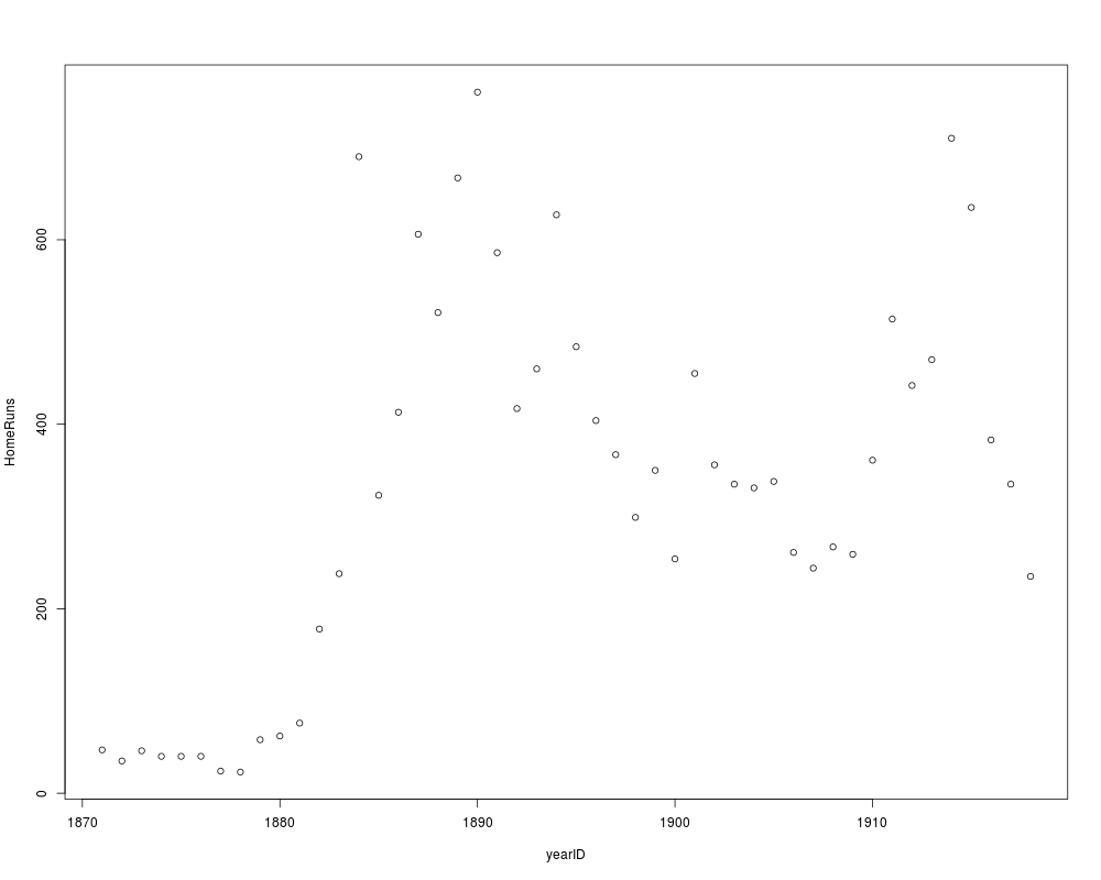
# after Chris Green,
# http://sabr.org/research/baseball-s-first-power-surge-home-runs-late-19th-century-major-leagues

# Total home runs by year
totalHR <- ddply(Batting, .(yearID), summarise,
                       HomeRuns = sum(as.numeric(HR), na.rm=TRUE),
                       Games = sum(as.numeric(G), na.rm=TRUE)
                       )

plot(HomeRuns ~ yearID, data=subset(totalHR, yearID<=1918))
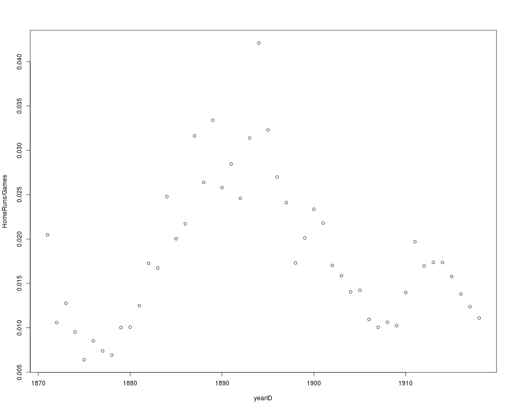
# take games into account?
plot(HomeRuns/Games ~ yearID, data=subset(totalHR, yearID<=1918))

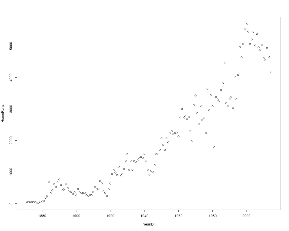
# long term trend?
plot(HomeRuns ~ yearID, data=totalHR)
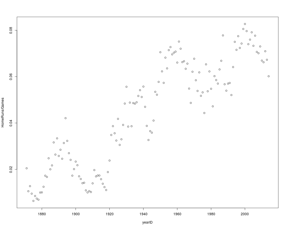
plot(HomeRuns/Games ~ yearID, data=totalHR)

Results

R version 3.3.1 (2016-06-21) -- "Bug in Your Hair"
Copyright (C) 2016 The R Foundation for Statistical Computing
Platform: x86_64-pc-linux-gnu (64-bit)

R is free software and comes with ABSOLUTELY NO WARRANTY.
You are welcome to redistribute it under certain conditions.
Type 'license()' or 'licence()' for distribution details.

R is a collaborative project with many contributors.
Type 'contributors()' for more information and
'citation()' on how to cite R or R packages in publications.

Type 'demo()' for some demos, 'help()' for on-line help, or
'help.start()' for an HTML browser interface to help.
Type 'q()' to quit R.

> library(Lahman)
> png(filename="/home/ddbj/snapshot/RGM3/R_CC/result/Lahman/Batting.Rd_%03d_medium.png", width=480, height=480)
> ### Name: Batting
> ### Title: Batting table
> ### Aliases: Batting
> ### Keywords: datasets
> 
> ### ** Examples
> 
> data(Batting)
> head(Batting)
   playerID yearID stint teamID lgID  G  AB  R  H X2B X3B HR RBI SB CS BB SO
1 abercda01   1871     1    TRO   NA  1   4  0  0   0   0  0   0  0  0  0  0
2  addybo01   1871     1    RC1   NA 25 118 30 32   6   0  0  13  8  1  4  0
3 allisar01   1871     1    CL1   NA 29 137 28 40   4   5  0  19  3  1  2  5
4 allisdo01   1871     1    WS3   NA 27 133 28 44  10   2  2  27  1  1  0  2
5 ansonca01   1871     1    RC1   NA 25 120 29 39  11   3  0  16  6  2  2  1
6 armstbo01   1871     1    FW1   NA 12  49  9 11   2   1  0   5  0  1  0  1
  IBB HBP SH SF GIDP
1  NA  NA NA NA   NA
2  NA  NA NA NA   NA
3  NA  NA NA NA   NA
4  NA  NA NA NA   NA
5  NA  NA NA NA   NA
6  NA  NA NA NA   NA
> require('plyr')
Loading required package: plyr
> 
> # calculate batting average and other stats
> batting <- battingStats()
> 
> # add salary to Batting data; need to match by player, year and team
> batting <- merge(batting, 
+                  Salaries[,c("playerID", "yearID", "teamID", "salary")], 
+                  by=c("playerID", "yearID", "teamID"), all.x=TRUE)
> 
> # Add name, age and bat hand information:
> masterInfo <- Master[, c('playerID', 'birthYear', 'birthMonth',
+                           'nameLast', 'nameFirst', 'bats')]
> batting <- merge(batting, masterInfo, all.x = TRUE)
> batting$age <- with(batting, yearID - birthYear -
+                              ifelse(birthMonth < 10, 0, 1))
> 
> batting <- arrange(batting, playerID, yearID, stint)
> 
> ## Generate a ggplot similar to the NYT graph in the story about Ted
> ## Williams and the last .400 MLB season 
> # http://www.nytimes.com/interactive/2011/09/18/sports/baseball/WILLIAMS-GRAPHIC.html
> 
> # Restrict the pool of eligible players to the years after 1899 and
> # players with a minimum of 450 plate appearances (this covers the
> # strike year of 1994 when Tony Gwynn hit .394 before play was suspended
> # for the season - in a normal year, the minimum number of plate appearances is 502)
> eligibleHitters <- subset(batting, yearID >= 1900 & PA > 450)
> 
> # Find the hitters with the highest BA in MLB each year (there are a
> # few ties).  Include all players with BA > .400
> topHitters <- ddply(eligibleHitters, .(yearID), subset, (BA == max(BA))|BA > .400)
> 
> # Create a factor variable to distinguish the .400 hitters
> topHitters$ba400 <- with(topHitters, BA >= 0.400)
> 
> # Sub-data frame for the .400 hitters plus the outliers after 1950
> # (averages above .380) - used to produce labels in the plot below
> bignames <- rbind(subset(topHitters, ba400),
+                   subset(topHitters, yearID > 1950 & BA > 0.380))
> # Cut to the relevant set of variables
> bignames <- subset(bignames, select = c('playerID', 'yearID', 'nameLast',
+                                         'nameFirst', 'BA'))
> 
> # Ditto for the original data frame
> topHitters <- subset(topHitters, select = c('playerID', 'yearID', 'BA', 'ba400'))
> 
> # Positional offsets to spread out certain labels
> #                     NL TC JJ TC GS TC RH GS HH RH RH BT TW TW  RC GB TG 
> bignames$xoffset <- c(0, 0, 0, 0, 0, 0, 0, 0, -8, 0, 3, 3, 0, 0, -2, 0, 0)
> bignames$yoffset <- c(0, 0, -0.003, 0, 0, 0, 0, 0, -0.004, 0, 0, 0, 0, 0, -0.003, 0, 0)  +  0.002
> 
> require('ggplot2')                               
Loading required package: ggplot2
> ggplot(topHitters, aes(x = yearID, y = BA)) +
+     geom_point(aes(colour = ba400), size = 2.5) +
+     geom_hline(yintercept = 0.400, size = 1) +
+     geom_text(data = bignames, aes(x = yearID + xoffset, y = BA + yoffset,
+                                    label = nameLast), size = 3) +
+     scale_colour_manual(values = c('FALSE' = 'black', 'TRUE' = 'red')) +
+     ylim(0.330, 0.430) +
+     xlab('Year') +
+     scale_y_continuous('Batting average',
+                        breaks = seq(0.34, 0.42, by = 0.02),
+                        labels = c('.340', '.360', '.380', '.400', '.420')) +
+     geom_smooth() +
+     theme(legend.position = 'none')
Scale for 'y' is already present. Adding another scale for 'y', which will
replace the existing scale.
> 
> ##########################################################
> # after Chris Green,
> # http://sabr.org/research/baseball-s-first-power-surge-home-runs-late-19th-century-major-leagues
> 
> # Total home runs by year
> totalHR <- ddply(Batting, .(yearID), summarise,
+                        HomeRuns = sum(as.numeric(HR), na.rm=TRUE),
+                        Games = sum(as.numeric(G), na.rm=TRUE)
+                        )
> 
> plot(HomeRuns ~ yearID, data=subset(totalHR, yearID<=1918))
> # take games into account?
> plot(HomeRuns/Games ~ yearID, data=subset(totalHR, yearID<=1918))
> 
> # long term trend?
> plot(HomeRuns ~ yearID, data=totalHR)
> plot(HomeRuns/Games ~ yearID, data=totalHR)
> 
> 
> 
> 
> 
> 
> 
> dev.off()
null device 
          1 
>