Supported by Dr. Osamu Ogasawara and  . . |
|
Last data update: 2014.03.03 |
Calculate metabolismDescriptionReturns daily time series of gross primary production (GPP), respiration (R), and net ecosystem production (NEP). Depending on the method used, other information may be returned as well. Calculations are made using one of 5 statistical methods. Usagemetab(data, method, wtr.name="wtr", irr.name="irr", do.obs.name="do.obs", ...) Arguments
ValueA data.frame containing columns for year, doy (day of year, julian day plus fraction of day), GPP, R, and NEP
Note that different models will have different attributes attached to them. See examples. Author(s)Ryan D. Batt See AlsoMetabolism models: metab.bookkeep, metab.ols, metab.mle, metab.kalman, metab.bayesian For smoothing noisy temperature: temp.kalman To calculate do.sat: o2.at.sat To calculate k.gas: k600.2.kGAS To calculate k600 values for k.gas: k.cole, k.crusius, k.macIntyre, k.read Examples
# fake data
datetime <- seq(as.POSIXct("2014-06-16 00:00:00", tz="GMT"),
as.POSIXct("2014-06-17 23:55:00", tz="GMT"), length.out=288*2)
do.obs <- 2*sin(2*pi*(1/288)*(1:(288*2))+1.1*pi) + 8 + rnorm(288*2, 0, 0.5)
wtr <- 3*sin(2*pi*(1/288)*(1:(288*2))+pi) + 17 + rnorm(288*2, 0, 0.15)
do.sat <- LakeMetabolizer:::o2.at.sat.base(wtr, 960)
irr <- (1500*sin(2*pi*(1/288)*(1:(288*2))+1.5*pi) +650 + rnorm(288*2, 0, 0.25)) *
ifelse(is.day(datetime, 42.3), 1, 0)
k.gas <- 0.4
z.mix <- 1
# plot time series
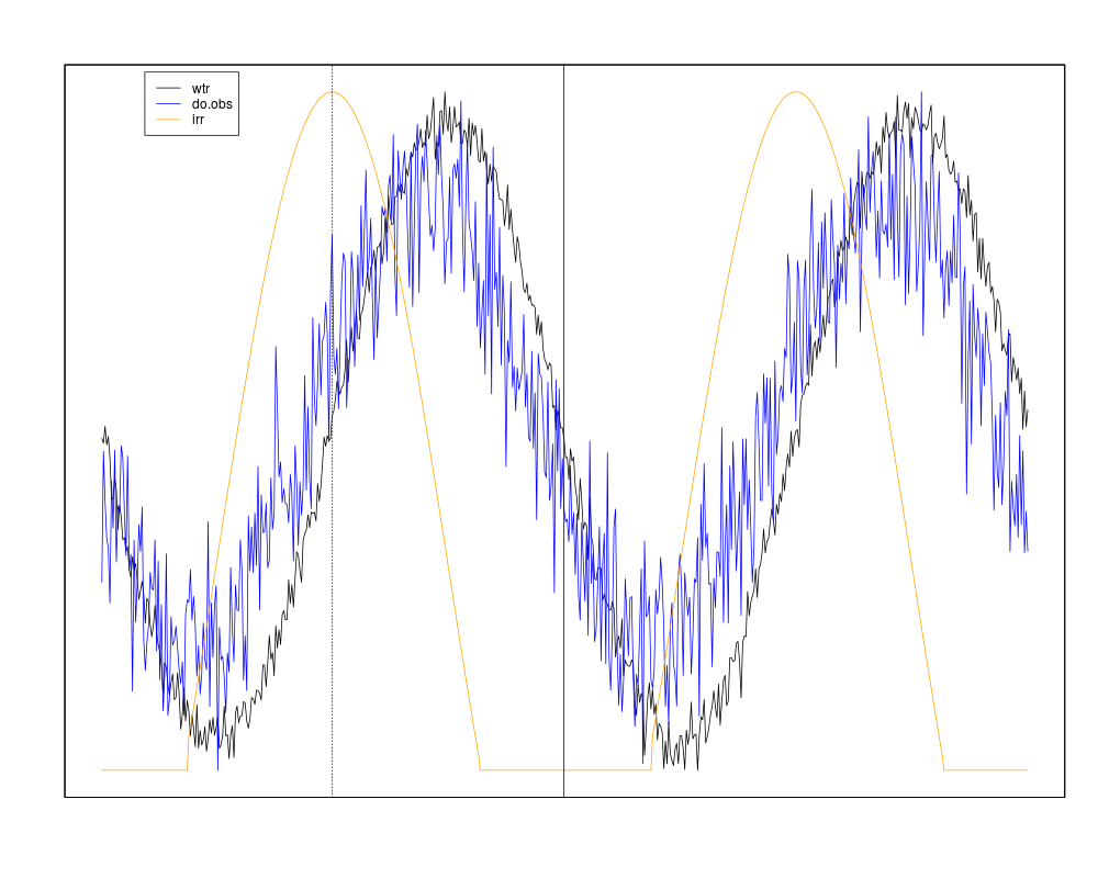
plot(wtr, type="l", xaxt="n", yaxt="n", xlab="", ylab="")
par(new=TRUE); plot(do.obs, type="l", col="blue", xaxt="n", yaxt="n", xlab="", ylab="")
par(new=TRUE); plot(irr, type="l", col="orange", xaxt="n", yaxt="n", xlab="", ylab="")
abline(v=144, lty="dotted")
abline(v=288)
legend("topleft", legend=c("wtr", "do.obs", "irr"), lty=1,
col=c("black", "blue", "orange"), inset=c(0.08, 0.01))
# put data in a data.frame
data <- data.frame(datetime=datetime, do.obs=do.obs, do.sat=do.sat, k.gas=k.gas,
z.mix=z.mix, irr=irr, wtr=wtr)
# run each metabolism model
m.bk <- metab(data, "bookkeep", lake.lat=42.6)
m.bk <- metab(data, lake.lat=42.6) # no method defaults to "bookeep"
m.ols <- metab(data, "ols", lake.lat=42.6)
m.mle <- metab(data, "mle", lake.lat=42.6)
m.kal <- metab(data, "kalman", lake.lat=42.6)
## Not run: m.bay <- metab(data, "bayesian", lake.lat=42.6)
# example attributes
names(attributes(m.ols))
attr(m.ols, "mod")
# To get full JAGS model
# including posterior draws:
## Not run: names(attributes(m.bay))
## Not run: attr(m.bay, "model")
Results
R version 3.3.1 (2016-06-21) -- "Bug in Your Hair"
Copyright (C) 2016 The R Foundation for Statistical Computing
Platform: x86_64-pc-linux-gnu (64-bit)

R is free software and comes with ABSOLUTELY NO WARRANTY.
You are welcome to redistribute it under certain conditions.
Type 'license()' or 'licence()' for distribution details.

R is a collaborative project with many contributors.
Type 'contributors()' for more information and
'citation()' on how to cite R or R packages in publications.

Type 'demo()' for some demos, 'help()' for on-line help, or
'help.start()' for an HTML browser interface to help.
Type 'q()' to quit R.

> library(LakeMetabolizer)
Loading required package: rLakeAnalyzer
> png(filename="/home/ddbj/snapshot/RGM3/R_CC/result/LakeMetabolizer/metab.Rd_%03d_medium.png", width=480, height=480)
> ### Name: metab
> ### Title: Calculate metabolism
> ### Aliases: metab
> ### Keywords: metabolism
>
> ### ** Examples
>
>
> # fake data
> datetime <- seq(as.POSIXct("2014-06-16 00:00:00", tz="GMT"),
+      as.POSIXct("2014-06-17 23:55:00", tz="GMT"), length.out=288*2)
> do.obs <- 2*sin(2*pi*(1/288)*(1:(288*2))+1.1*pi) + 8 + rnorm(288*2, 0, 0.5)
> wtr <- 3*sin(2*pi*(1/288)*(1:(288*2))+pi) + 17 + rnorm(288*2, 0, 0.15)
> do.sat <- LakeMetabolizer:::o2.at.sat.base(wtr, 960)
> irr <- (1500*sin(2*pi*(1/288)*(1:(288*2))+1.5*pi) +650 + rnorm(288*2, 0, 0.25)) *
+      ifelse(is.day(datetime, 42.3), 1, 0)
> k.gas <- 0.4
> z.mix <- 1
>
> # plot time series
> plot(wtr, type="l", xaxt="n", yaxt="n", xlab="", ylab="")
> par(new=TRUE); plot(do.obs, type="l", col="blue", xaxt="n", yaxt="n", xlab="", ylab="")
> par(new=TRUE); plot(irr, type="l", col="orange", xaxt="n", yaxt="n", xlab="", ylab="")
> abline(v=144, lty="dotted")
> abline(v=288)
> legend("topleft", legend=c("wtr", "do.obs", "irr"), lty=1,
+      col=c("black", "blue", "orange"), inset=c(0.08, 0.01))
>
> # put data in a data.frame
> data <- data.frame(datetime=datetime, do.obs=do.obs, do.sat=do.sat, k.gas=k.gas,
+      z.mix=z.mix, irr=irr, wtr=wtr)
>
> # run each metabolism model
> m.bk <- metab(data, "bookkeep", lake.lat=42.6)
[1] "Points removed due to incomplete day or duplicated time step: 0"
[1] "NA's added to fill in time series: 0"
>  m.bk <- metab(data, lake.lat=42.6) # no method defaults to "bookeep"
[1] "Points removed due to incomplete day or duplicated time step: 0"
[1] "NA's added to fill in time series: 0"
> m.ols <- metab(data, "ols", lake.lat=42.6)
[1] "Points removed due to incomplete day or duplicated time step: 0"
[1] "NA's added to fill in time series: 0"
> m.mle <- metab(data, "mle", lake.lat=42.6)
[1] "Points removed due to incomplete day or duplicated time step: 0"
[1] "NA's added to fill in time series: 0"
> m.kal <- metab(data, "kalman", lake.lat=42.6)
[1] "Points removed due to incomplete day or duplicated time step: 0"
[1] "NA's added to fill in time series: 0"
> ## Not run: m.bay <- metab(data, "bayesian", lake.lat=42.6)
>
> # example attributes
> names(attributes(m.ols))
[1] "names"     "row.names" "class"     "mod"
> attr(m.ols, "mod")
[[1]]

Call:
lm(formula = noflux.do.diff ~ irr[-nobs] + lntemp[-nobs] - 1)

Coefficients:
   irr[-nobs]  lntemp[-nobs]
    3.208e-05     -9.913e-03


[[2]]

Call:
lm(formula = noflux.do.diff ~ irr[-nobs] + lntemp[-nobs] - 1)

Coefficients:
   irr[-nobs]  lntemp[-nobs]
    2.993e-05     -8.424e-03


>
> # To get full JAGS model
> # including posterior draws:
> ## Not run: names(attributes(m.bay))
> ## Not run: attr(m.bay, "model")
>
>
>
>
>
>
> dev.off()
null device
          1
>
|