MedCouple Estimator

Description

A robust measure of asymmetry. See References for details.

Usage

medcouple_estimator(x, seed = sample.int(1e+06, 1))

Arguments

Value

float; measures the degree of asymmetry

References

Brys, G., M. Hubert, and A. Struyf (2004). “A robust measure of skewness”. Journal of Computational and Graphical Statistics 13 (4), 996 - 1017.

See Also

test_symmetry

Examples

# a simulation
kNumSim <- 100
kNumObs <- 200

################# Gaussian (Symmetric) #### 
A <- t(replicate(kNumSim, {xx <- rnorm(kNumObs); c(skewness(xx), medcouple_estimator(xx))}))
########### skewed LambertW x Gaussian #### 
tau.s <- gamma_01(0.2) # zero mean, unit variance, but positive skewness
rbind(mLambertW(theta = list(beta = tau.s[c("mu_x", "sigma_x")], 
                             gamma = tau.s["gamma"]), 
                distname="normal"))
B <- t(replicate(kNumSim, 
                 {
                   xx <- rLambertW(n = kNumObs, 
                                   theta = list(beta = tau.s[c("mu_x", "sigma_x")], 
                                                gamma = tau.s["gamma"]), 
                                   distname="normal")
                   c(skewness(xx), medcouple_estimator(xx))
                 }))
                  
colnames(A) <- colnames(B) <- c("MedCouple", "Pearson Skewness")

layout(matrix(1:4, ncol = 2))
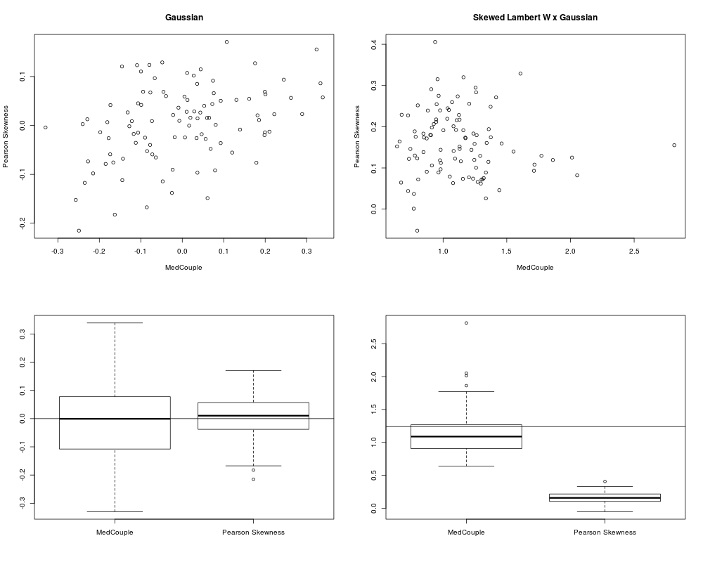
plot(A, main = "Gaussian")
boxplot(A)
abline(h = 0)

plot(B, main = "Skewed Lambert W x Gaussian")
boxplot(B)
abline(h = mLambertW(theta = list(beta = tau.s[c("mu_x", "sigma_x")], 
                                  gamma = tau.s["gamma"]), 
                     distname="normal")["skewness"])

colMeans(A)
apply(A, 2, sd)

colMeans(B)
apply(B, 2, sd)

Results

R version 3.3.1 (2016-06-21) -- "Bug in Your Hair"
Copyright (C) 2016 The R Foundation for Statistical Computing
Platform: x86_64-pc-linux-gnu (64-bit)

R is free software and comes with ABSOLUTELY NO WARRANTY.
You are welcome to redistribute it under certain conditions.
Type 'license()' or 'licence()' for distribution details.

R is a collaborative project with many contributors.
Type 'contributors()' for more information and
'citation()' on how to cite R or R packages in publications.

Type 'demo()' for some demos, 'help()' for on-line help, or
'help.start()' for an HTML browser interface to help.
Type 'q()' to quit R.

> library(LambertW)
Loading required package: MASS
Loading required package: ggplot2
This is 'LambertW' version 0.6.4.  Please see the NEWS file and citation("LambertW").

> png(filename="/home/ddbj/snapshot/RGM3/R_CC/result/LambertW/medcouple_estimator.Rd_%03d_medium.png", width=480, height=480)
> ### Name: medcouple_estimator
> ### Title: MedCouple Estimator
> ### Aliases: medcouple_estimator
> ### Keywords: univar
> 
> ### ** Examples
> 
> 
> # a simulation
> kNumSim <- 100
> kNumObs <- 200
> 
> ################# Gaussian (Symmetric) #### 
> A <- t(replicate(kNumSim, {xx <- rnorm(kNumObs); c(skewness(xx), medcouple_estimator(xx))}))
> ########### skewed LambertW x Gaussian #### 
> tau.s <- gamma_01(0.2) # zero mean, unit variance, but positive skewness
> rbind(mLambertW(theta = list(beta = tau.s[c("mu_x", "sigma_x")], 
+                              gamma = tau.s["gamma"]), 
+                 distname="normal"))
     mean          sd skewness kurtosis
[1,] -2.775558e-17 1  1.240552 5.692398
> B <- t(replicate(kNumSim, 
+                  {
+                    xx <- rLambertW(n = kNumObs, 
+                                    theta = list(beta = tau.s[c("mu_x", "sigma_x")], 
+                                                 gamma = tau.s["gamma"]), 
+                                    distname="normal")
+                    c(skewness(xx), medcouple_estimator(xx))
+                  }))
>                   
> colnames(A) <- colnames(B) <- c("MedCouple", "Pearson Skewness")
> 
> layout(matrix(1:4, ncol = 2))
> plot(A, main = "Gaussian")
> boxplot(A)
> abline(h = 0)
> 
> plot(B, main = "Skewed Lambert W x Gaussian")
> boxplot(B)
> abline(h = mLambertW(theta = list(beta = tau.s[c("mu_x", "sigma_x")], 
+                                   gamma = tau.s["gamma"]), 
+                      distname="normal")["skewness"])
> 
> colMeans(A)
       MedCouple Pearson Skewness 
   -0.0010908342     0.0007825742 
> apply(A, 2, sd)
       MedCouple Pearson Skewness 
      0.18404815       0.08442167 
> 
> colMeans(B)
       MedCouple Pearson Skewness 
       1.1723081        0.1670144 
> apply(B, 2, sd)
       MedCouple Pearson Skewness 
      0.36811159       0.08182489 
> 
> 
> 
> 
> 
> 
> dev.off()
null device 
          1 
>