R Graphical Manual

Browse All

Last data update: 2014.03.03

R: Visual and statistical Gaussianity check

test_normality

R Documentation

Visual and statistical Gaussianity check

Description

Graphical and statistical check if data is Gaussian (three common Normality tests, QQ-plots, histograms, etc).

test_normality does not show the autocorrelation function (ACF) estimate for lag 0, since it always equals 1. Thus removing it does not lose any information, but greatly improves the y-axis scale for higher order lags (which are usually very small compared to 1).

test_norm is a shortcut for test_normality.

Usage

test_normality(data, show.volatility = FALSE, plot = TRUE, pch = 1,
  add.legend = TRUE, seed = sample(1e+06, 1))

test_norm(...)

Arguments

`data`	a numeric vector of data values.
`show.volatility`	logical; if `TRUE` the squared (centered) data and its ACF are also shown. Useful for time series data to see if squares exhibit dependence (for financial data they typically do); default: `FALSE`.
`plot`	Should visual checks (histogram, densities, qqplot, ACF) be plotted? Default `TRUE`; otherwise only hypothesis test results are returned.
`pch`	a vector of plotting characters or symbols; default `pch = 1`.
`add.legend`	logical; if `TRUE` (default) a legend is placed in histogram/density plot.
`seed`	optional; if sample size > 5,000, then some normality tests fail to run. In this case it uses a subsample of size 5,000. For reproducibility, the seed can be specified by user. By default it uses a random seed.
`...`	arguments as in `test_normality`.

Value

A list with results of 3 normality tests (each of class htest) and the seed used for subsampling:

`anderson.darling`	Anderson Darling (if nortest package is available),
`shapiro.francia`	Shapiro-Francia (if nortest package is available),
`shapiro.wilk`	Shapiro-Wilk,
`seed`	seed for subsampling (only used if sample size > 5,000).

References

Thode Jr., H.C. (2002): “Testing for Normality”. Marcel Dekker, New York.

Examples


y <- rLambertW(n = 1000, theta = list(beta = c(3, 4), gamma = 0.3),
               distname = "normal")
test_normality(y)

x <- rnorm(n = 1000)
test_normality(x)

# mixture of exponential and normal
test_normality(c(rexp(100), rnorm(100, mean = -5)))

Results


R version 3.3.1 (2016-06-21) -- "Bug in Your Hair"
Copyright (C) 2016 The R Foundation for Statistical Computing
Platform: x86_64-pc-linux-gnu (64-bit)

R is free software and comes with ABSOLUTELY NO WARRANTY.
You are welcome to redistribute it under certain conditions.
Type 'license()' or 'licence()' for distribution details.

R is a collaborative project with many contributors.
Type 'contributors()' for more information and
'citation()' on how to cite R or R packages in publications.

Type 'demo()' for some demos, 'help()' for on-line help, or
'help.start()' for an HTML browser interface to help.
Type 'q()' to quit R.

> library(LambertW)
Loading required package: MASS
Loading required package: ggplot2
This is 'LambertW' version 0.6.4.  Please see the NEWS file and citation("LambertW").

> png(filename="/home/ddbj/snapshot/RGM3/R_CC/result/LambertW/test_normality.Rd_%03d_medium.png", width=480, height=480)
> ### Name: test_normality
> ### Title: Visual and statistical Gaussianity check
> ### Aliases: test_norm test_normality
> ### Keywords: hplot htest
> 
> ### ** Examples
> 
> 
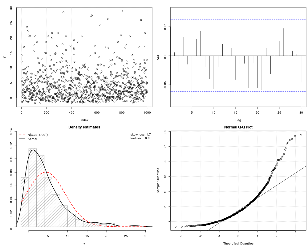
> y <- rLambertW(n = 1000, theta = list(beta = c(3, 4), gamma = 0.3),
+                distname = "normal")
> test_normality(y)
$seed
[1] 887720

$shapiro.wilk

	Shapiro-Wilk normality test

data:  data.test
W = 0.87294, p-value < 2.2e-16


$shapiro.francia

	Shapiro-Francia normality test

data:  data.test
W = 0.87256, p-value < 2.2e-16


$anderson.darling

	Anderson-Darling normality test

data:  data
A = 33.294, p-value < 2.2e-16


> 
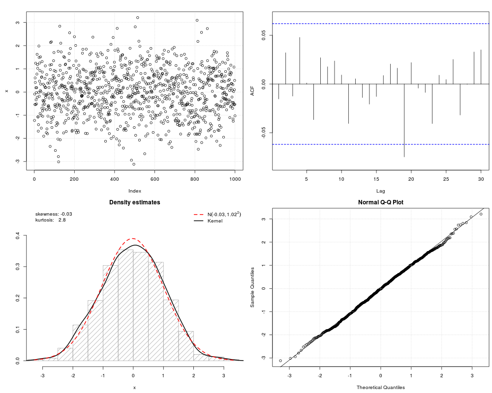
> x <- rnorm(n = 1000)
> test_normality(x)
$seed
[1] 801073

$shapiro.wilk

	Shapiro-Wilk normality test

data:  data.test
W = 0.99694, p-value = 0.05206


$shapiro.francia

	Shapiro-Francia normality test

data:  data.test
W = 0.99698, p-value = 0.05304


$anderson.darling

	Anderson-Darling normality test

data:  data
A = 0.64439, p-value = 0.09253


> 
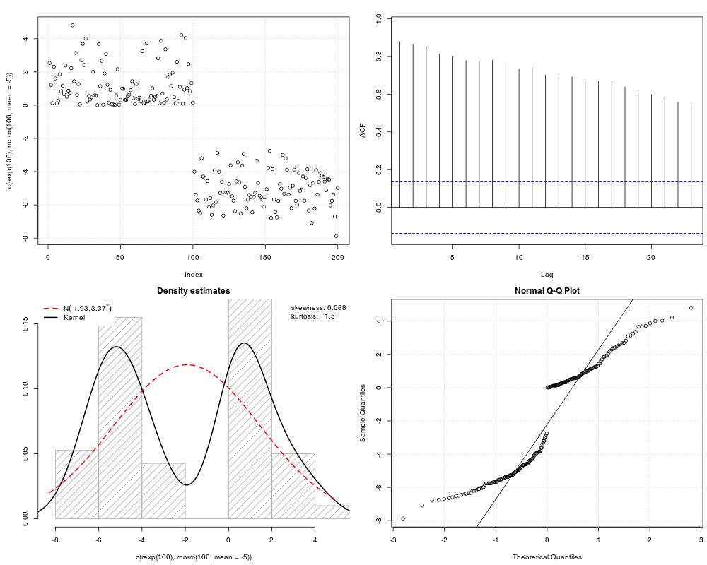
> # mixture of exponential and normal
> test_normality(c(rexp(100), rnorm(100, mean = -5)))
$seed
[1] 899389

$shapiro.wilk

	Shapiro-Wilk normality test

data:  data.test
W = 0.88261, p-value = 2.242e-11


$shapiro.francia

	Shapiro-Francia normality test

data:  data.test
W = 0.88611, p-value = 7.808e-10


$anderson.darling

	Anderson-Darling normality test

data:  data
A = 11.329, p-value < 2.2e-16


> 
> 
> 
> 
> 
> 
> dev.off()
null device 
          1 
>