a vector containing the time series or a time-series object.
bins
a scalar denoting the number of bins to calculate the
conditional moments on.
steps
a vector giving the τ steps to calculate the
conditional moments (in samples (=τ * sf)).
sf
a scalar denoting the sampling frequency (optional if data
is a time-series object).
bin_min
a scalar denoting the minimal number of events per bin.
Defaults to 100.
reqThreads
a scalar denoting how many threads to use. Defaults to
-1 which means all available cores.
Value
Langevin1D returns a list with thirteen components:
D1
a vector of the Drift coefficient for each bin.
eD1
a vector of the error of the Drift coefficient for each
bin.
D2
a vector of the Diffusion coefficient for each bin.
eD2
a vector of the error of the Driffusion coefficient for
each bin.
D4
a vector of the fourth Kramers-Moyal coefficient for each
bin.
mean_bin
a vector of the mean value per bin.
density
a vector of the number of events per bin.
M1
a matrix of the first conditional moment for each
τ. Rows corespond to bin, columns to τ.
eM1
a matrix of the error of the first conditional moment
for each τ. Rows corespond to bin, columns to τ.
M2
a matrix of the second conditional moment for each
τ. Rows corespond to bin, columns to τ.
eM2
a matrix of the error of the second conditional moment
for each τ. Rows corespond to bin, columns to τ.
M4
a matrix of the fourth conditional moment for each
τ. Rows corespond to bin, columns to τ.
U
a vector of the bin borders.
Author(s)
Philip Rinn
See Also
Langevin2D
Examples
# Set number of bins, steps and the sampling frequency
bins <- 20;
steps <- c(1:5);
sf <- 1000;
#### Linear drift, constant diffusion
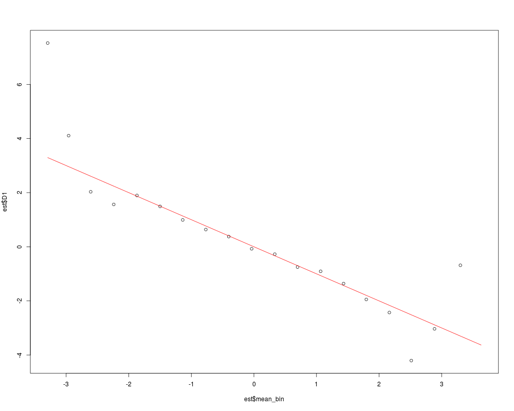
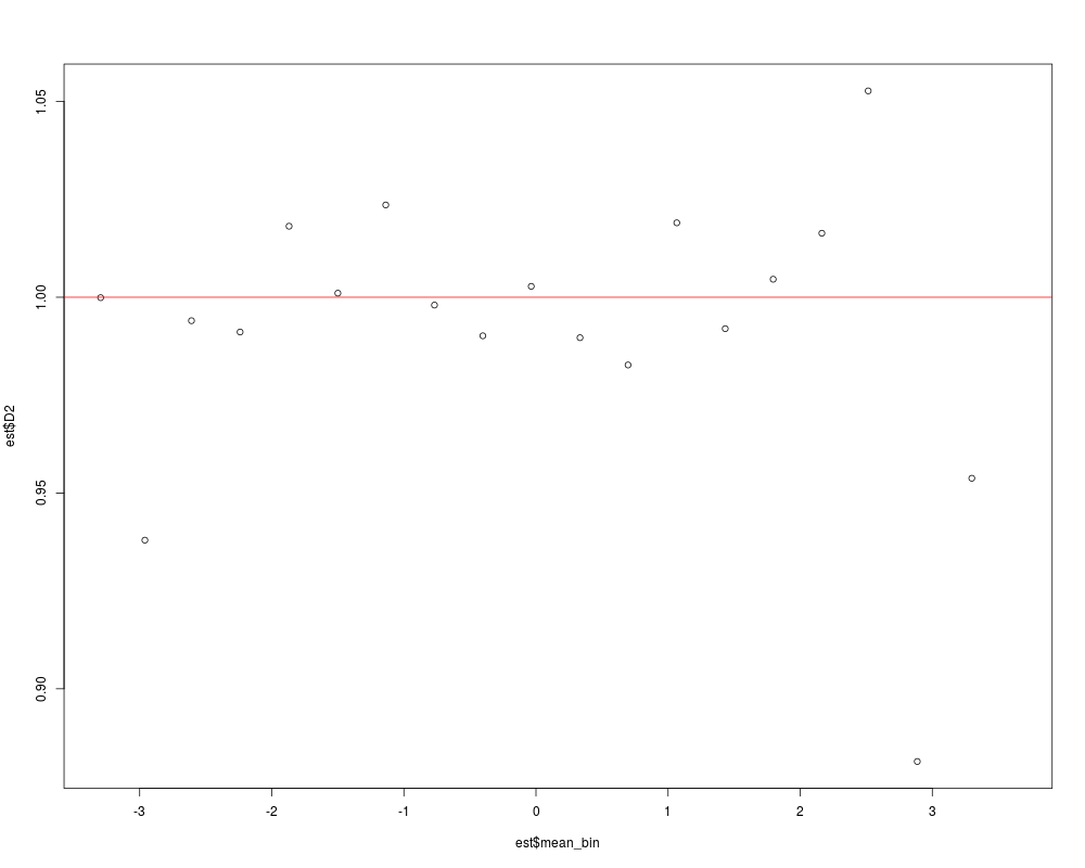
# Generate a time series with linear D^1 = -x and constant D^2 = 1
x <- timeseries1D(N=1e6, d11=-1, d20=1, sf=sf);
# Do the analysis
est <- Langevin1D(x, bins, steps, sf, reqThreads=2);
# Plot the result and add the theoretical expectation as red line
plot(est$mean_bin, est$D1);
lines(est$mean_bin, -est$mean_bin, col='red');
plot(est$mean_bin, est$D2);
abline(h=1, col='red');
#### Cubic drift, constant diffusion
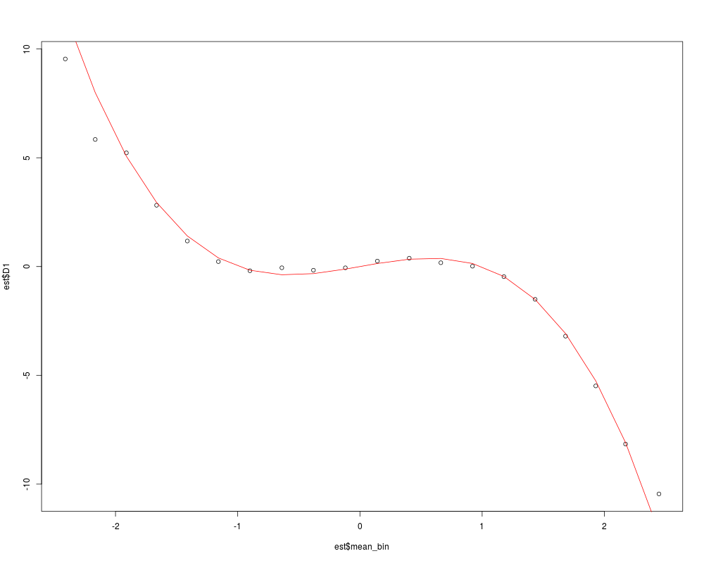
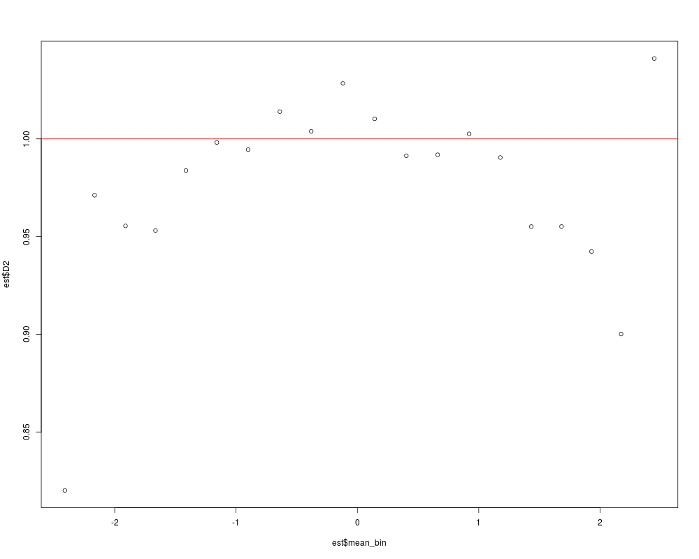
# Generate a time series with cubic D^1 = x - x^3 and constant D^2 = 1
x <- timeseries1D(N=1e6, d13=-1, d11=1, d20=1, sf=sf);
# Do the analysis
est <- Langevin1D(x, bins, steps, sf, reqThreads=2);
# Plot the result and add the theoretical expectation as red line
plot(est$mean_bin, est$D1);
lines(est$mean_bin, est$mean_bin - est$mean_bin^3, col='red');
plot(est$mean_bin, est$D2);
abline(h=1, col='red');
Results
R version 3.3.1 (2016-06-21) -- "Bug in Your Hair"
Copyright (C) 2016 The R Foundation for Statistical Computing
Platform: x86_64-pc-linux-gnu (64-bit)

R is free software and comes with ABSOLUTELY NO WARRANTY.
You are welcome to redistribute it under certain conditions.
Type 'license()' or 'licence()' for distribution details.

R is a collaborative project with many contributors.
Type 'contributors()' for more information and
'citation()' on how to cite R or R packages in publications.

Type 'demo()' for some demos, 'help()' for on-line help, or
'help.start()' for an HTML browser interface to help.
Type 'q()' to quit R.

> library(Langevin)
> png(filename="/home/ddbj/snapshot/RGM3/R_CC/result/Langevin/Langevin1D.Rd_%03d_medium.png", width=480, height=480)
> ### Name: Langevin1D
> ### Title: Calculate the Drift and Diffusion of one-dimensional stochastic
> ###   processes
> ### Aliases: Langevin1D
>
> ### ** Examples
>
> # Set number of bins, steps and the sampling frequency
> bins <- 20;
> steps <- c(1:5);
> sf <- 1000;
>
> #### Linear drift, constant diffusion
>
> # Generate a time series with linear D^1 = -x and constant D^2 = 1
> x <- timeseries1D(N=1e6, d11=-1, d20=1, sf=sf);
> # Do the analysis
> est <- Langevin1D(x, bins, steps, sf, reqThreads=2);
> # Plot the result and add the theoretical expectation as red line
> plot(est$mean_bin, est$D1);
> lines(est$mean_bin, -est$mean_bin, col='red');
> plot(est$mean_bin, est$D2);
> abline(h=1, col='red');
>
> #### Cubic drift, constant diffusion
>
> # Generate a time series with cubic D^1 = x - x^3 and constant D^2 = 1
> x <- timeseries1D(N=1e6, d13=-1, d11=1, d20=1, sf=sf);
> # Do the analysis
> est <- Langevin1D(x, bins, steps, sf, reqThreads=2);
> # Plot the result and add the theoretical expectation as red line
> plot(est$mean_bin, est$D1);
> lines(est$mean_bin, est$mean_bin - est$mean_bin^3, col='red');
> plot(est$mean_bin, est$D2);
> abline(h=1, col='red');
>
>
>
>
>
> dev.off()
null device
          1
>
 .
.