Supported by Dr. Osamu Ogasawara and  . . |
|
Last data update: 2014.03.03 |
Functions for generating a multiresolution, compactly supported basis, multiresolution covariance functions and simulating from these processes.DescriptionThese functions support the Usage# LKrig.cov(x1, x2 = NULL, LKinfo, C = NA, marginal = FALSE) LKrig.cov.plot( LKinfo, NP=200, center = NULL, xlim = NULL, ylim = NULL) LKrigCovWeightedObs(x1, wX, LKinfo) LKrig.basis(x1, LKinfo, verbose = FALSE) LKrig.precision(LKinfo, return.B = FALSE, verbose=FALSE) LKrig.quadraticform( Q, PHI, choleskyMemory = NULL) LKrig.spind2spam(obj, add.zero.rows=TRUE) LKrigMarginalVariance(x1, LKinfo, verbose = FALSE) Arguments
DetailsThe basis functions are two-dimensional radial basis functions based on the compactly supported stationary covariance function (Wendland covariance) and centered on regular grid points with the scaling tied to the grid spacing. For a basis at the coarsest level, the grid centers are generated by expanding the two sequences seq(grid.info$xmin,grid.info$xmax,grid.info$delta) seq(grid.info$ymin,grid.info$ymax,grid.info$delta) into a regular grid of center points. The same spacing
 centers<- expand.grid(seq(xmin,xmax,delta),
                       seq(ymin,ymax,delta) )
 bigD<- rdist( x1, centers)/(delta*2.5)
 PHI<- Wendland.function( bigD)
Note that there will be The basis functions are then normalized by scaling the basis functions at each location so that resulting marginal variance of the process is 1. This is done to coax the covariance model closer to a stationary representation. It is easiest to express this normalization by pseudo R code: If Omega<- solve(Q) process.variance <- diag(PHI%*% Omega %*%t(PHI) ) PHI.normalized <- diag(1/sqrt(process.variance)) %*% PHI where Although correct, the code above is not an efficient algorithm to
compute the unnormalized process variance. First the normalization
can be done level by level rather than dealing with the entire
multiresolution process at once. Also it is important to work with the
precision matrix rather than the covariance. The function
The precision matrix for the basis coefficients at each resolution has
the form Below we give more details on how the weights are determined. Following the notation in Lindgren and Rue a.wght= 4 + k2 with k2 greater than or equal to 0. Some schematics for filling in the B matrix are given below (values are weights for the SAR on the lattice with a period indicating zero weights).
                                                 __________
   .   -1     .         |  -1      .            |  a.wght  -1
                        |                       |
  -1  a.wght  -1        | a.wght   -1           |   -1      .
                        |                       |
   .  -1      .         |  -1      .            |    .      .

Interior point        Left edge              Upper left corner
Previous versions of LatticeKrig considered an edge correction to reflect other boundary conditions. We have found these corrections to be numerically unstable, however, and so prefer at this time of writing adding a buffer of lattice points and using the uncorrected weights described above. ValueLKrig.basis: A matrix with number of rows equal to the rows of
LKrig.precision: For LKrig.cov: If LKrigMarginalVariance: Gives the marginal variance of the
LatticeKrig process at each level and at the locations in LKrig.sim: A matrix with dimensions of LKrig.cov.plot: Evaluates the covariance specified in the list
LKinfo with respect to the point out<- LKrig.cov.plot(LKinfo) matplot( out$d, out$cov, type="l") LKrig.quadraticform: Returns a vector that is
LKrig.normalize.basis, LKrig.normalize.basis.fast, LKrig.normalize.basis.slow: A vector of variances corresponding to the unnormalized process at the locations. LKrig.spind2spam: This converts a matrix in spind sparse format to spam sparse format. Although useful for checking, LatticeKrig now uses the
the
and
give the same result. Author(s)Doug Nychka See AlsoLKrig, mKrig, Krig, fastTps, Wendland, LKrigSAR Examples
# Load ozone data set
data(ozone2)
x<-ozone2$lon.lat
y<- ozone2$y[16,]
# Find location that are not 'NA'.
# (LKrig is not set up to handle missing observations.)
good <- !is.na( y)
x<- x[good,]
y<- y[good]
LKinfo<- LKrigSetup( x,NC=20,nlevel=1, alpha=1, lambda= .3 , a.wght=5)
# BTW lambda is close to MLE
# What does the LatticeKrig covariance function look like?
# set up LKinfo object
# NC=10 sets the grid for the first level of basis functions
# NC^2 = 100 grid points in first level if square domain.
# given four levels the number of basis functions
# = 10^2 + 19^2 +37^2 + 73^2 = 5329
# effective range scales as roughly kappa where a.wght = 4 + kappa^2
# or exponential decreasing marginal variances for the components.
NC<- 10
nlevel<- 4
a.wght<- rep( 4 + 1/(.5)^2, nlevel)
alpha<- 1/2^(0:(nlevel-1))
LKinfo2<- LKrigSetup( cbind( c( -1,1), c(-1,1)), NC=NC,
nlevel=nlevel, a.wght=a.wght,alpha=alpha)
# evaluate covariance along the horizontal line through
# midpoint of region -- (0,0) in this case.
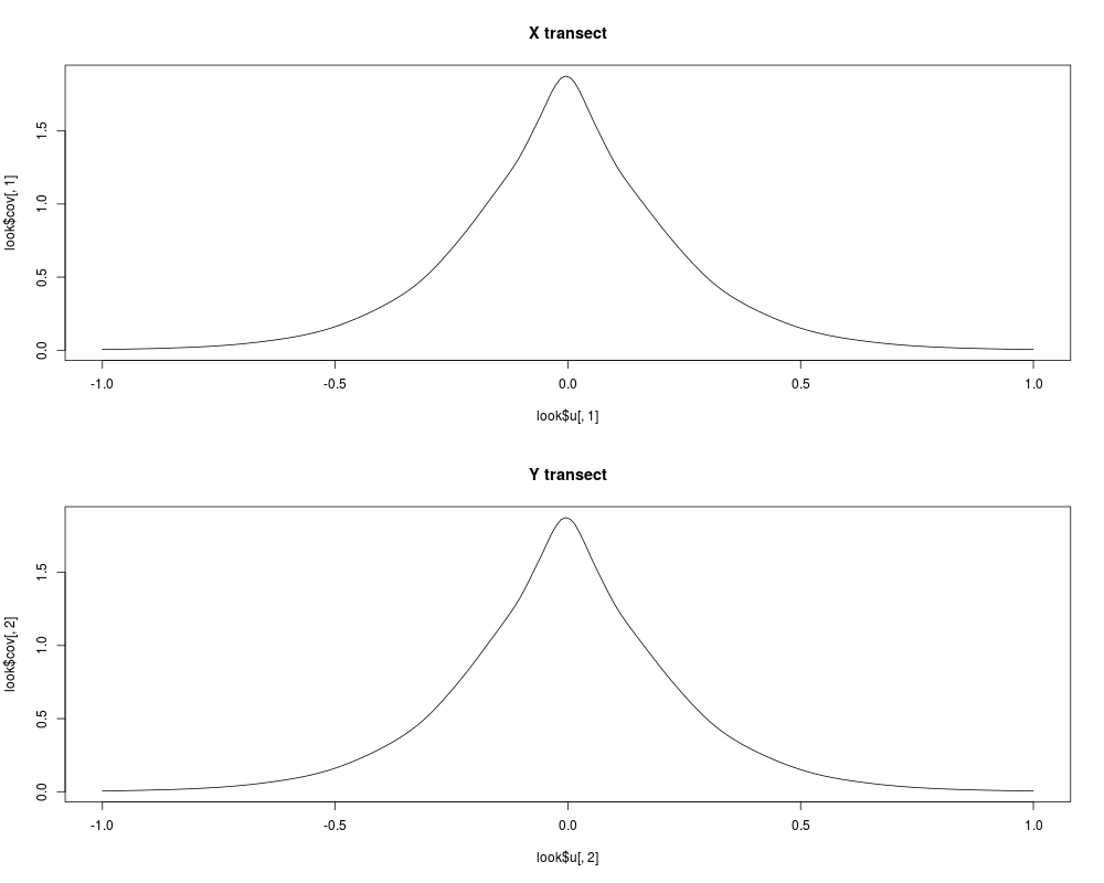
look<- LKrig.cov.plot( LKinfo2)
# a plot of the covariance function in x and y with respect to (0,0)
set.panel(2,1)
plot(look$u[,1], look$cov[,1], type="l")
title("X transect")
plot(look$u[,2], look$cov[,2], type="l")
title("Y transect")
set.panel(1,1)
#
#
## Not run:
# full 2-d view of the covariance (this example follows the code
# in LKrig.cov.plot)
x2<- cbind( 0,0)
x1<- make.surface.grid( list(x=seq( -1,1,,40), y=seq( -1,1,,40)))
look<- LKrig.cov( x1,x2, LKinfo2)
contour( as.surface( x1, look))
# Note nearly circular contours.
# of course plot(look[,80/2]) should look like plot above.
#
## End(Not run)
## Not run:
#Some correlation functions from different models
set.panel(2,1)
# a selection of ranges:
hold<- matrix( NA, nrow=150, ncol=4)
kappa<- seq( .25,1,,4)
x2<- cbind( 0,0)
x1<- cbind( seq(-1,1,,150), rep( 0,150))
for( k in 1:4){
LKtemp<- LKrigSetup( cbind( c( -1,1), c(-1,1)), NC=NC,
nlevel=nlevel,
a.wght= 4 + 1/(kappa[k]^2),
alpha=alpha)
hold[,k]<- LKrig.cov( x1,x2, LKinfo=LKtemp)
}
matplot( x1[,1], hold, type="l", lty=1, col=rainbow(5), pch=16 )
# a selection of smoothness parameters
ktemp<- .5 # fix range
alpha.power<- seq( 1,4,,4)
LKtemp<- LKinfo2
for( k in 1:4){
LKtemp<- LKrigSetup( cbind( c( -1,1), c(-1,1)), NC=NC,
nlevel=nlevel,
a.wght= 4 + 1/(ktemp^2),
alpha=alpha^alpha.power[k])
hold[,k]<- LKrig.cov( x1,x2, LKinfo=LKtemp)
}
matplot( x1[,1], hold, type="l", lty=1, col=rainbow(5) )
set.panel()
## End(Not run)
## Not run:
# generating a basis on the domain [-1,1] by [-1,1] with 1 level
# Default number of buffer points are added to each side.
LKinfo<- LKrigSetup(cbind( c(-1,1), c(-1,1)), NC=6,
nlevel=1, a.wght=4.5,alpha=1, NC.buffer=0 )
# evaluate the basis functions on a grid to look at them
xg<- make.surface.grid( list(x=seq(-1,1,,50), y= seq(-1,1,,50)))
PHI<- LKrig.basis( xg,LKinfo)
dim(PHI) # should be 2500=50^2 by 36=6^2
# plot the 9th basis function as.surface is a handy function to
# reformat the vector as an image object
# using the grid information in an attribute of the grid points
set.panel(1,3)
image.plot(as.surface(xg, PHI[,9]))
points( make.surface.grid( LKrigLatticeCenters(LKinfo, 1)) , col="grey", cex=.5)
title("A radial basis function")
# compare to the tensor product basis type
LKinfo2<- LKrigSetup(cbind( c(-1,1), c(-1,1)), NC=6,
nlevel=1, a.wght=4.5,alpha=1, NC.buffer=0,
BasisType="Tensor" )
PHI2<- LKrig.basis( xg,LKinfo2)
image.plot(as.surface(xg, PHI2[,9]))
points( make.surface.grid( LKrigLatticeCenters(LKinfo, 1)), col="grey", cex=.5)
title("Tensor product basis function")
image.plot(as.surface(xg, PHI[,9] - PHI2[,9]))
points( make.surface.grid( LKrigLatticeCenters(LKinfo, 1)), col="grey", cex=.5)
title(" Radial - Tensor for 9th basis function")
set.panel()
## End(Not run)
#
# example of basis function indexing
#
## Not run:
# generating a basis on the domain [-1,1]X[-1,1] with 3 levels
# note that there are no buffering grid points.
set.panel(3,2)
LKinfo<-LKrigSetup(cbind( c(-1,1), c(-1,1)), NC=6,
a.wght=rep(5,3), alpha=c(1,.5,.25), nlevel=3,
NC.buffer=0)
# evaluate the basis functions on a grid to look at them
xtemp<- seq(-1,1,,40)
xg<- make.surface.grid( list(x=xtemp, y= xtemp) )
PHI<- LKrig.basis( xg,LKinfo)
# coerce to dense matrix format to make plotting easier.
PHI<- spam2full(PHI)
# first tenth, and last basis function in each resolution level
# basis functions centers are added
set.panel(3,3)
for( j in 1:3){
id1<- LKinfo$latticeInfo$offset[j]+ 1
id2<- LKinfo$latticeInfo$offset[j]+ 10
idlast<- LKinfo$latticeInfo$offset[j] +
LKinfo$latticeInfo$mx[j,1]*LKinfo$latticeInfo$mx[j,2]
centers<- make.surface.grid(LKrigLatticeCenters(LKinfo, j) )
image.plot( as.surface(xg, PHI[,id1]))
points( centers, cex=.2, col="grey")
image.plot(as.surface(xg, PHI[,id2]))
points( centers, cex=.2, col="grey")
image.plot( as.surface(xg, PHI[,idlast]))
points( centers, cex=.2, col="grey")
}
set.panel()
## End(Not run)
## Not run:
# examining the stationarity of covariance model
temp.fun<-
function( NC.buffer=0, NC=4, a.wght=4.01){
LKinfo<- LKrigSetup(cbind( c(-1,1), c(-1,1)),nlevel=1, alpha=1,
a.wght=a.wght, NC=NC,
NC.buffer=NC.buffer,
choleskyMemory=list(nnzR=2e6))
cov1y<- cov1x<- cov0x<- cov0y<- matrix( NA, nrow=200, ncol=20)
cov1dx<- cov1dy<- cov0dx<- cov0dy<- matrix( NA, nrow=200, ncol=20)
cgrid<- seq( 0,1,,20)
for( k in 1:20){
hold<- LKrig.cov.plot( LKinfo,
center=rbind( c(cgrid[k], cgrid[k])), NP=200)
cov1x[,k] <- hold$cov[,1]
cov1y[,k] <- hold$cov[,2]
cov1dx[,k] <- hold$d[,1]
cov1dy[,k] <- hold$d[,2]
hold<- LKrig.cov.plot( LKinfo,
center=rbind( c(cgrid[k],0) ), NP=200)
cov0x[,k] <- hold$cov[,1]
cov0y[,k] <- hold$cov[,2]
cov0dx[,k] <- hold$d[,1]
cov0dy[,k] <- hold$d[,2]
}
matplot( cov1dx, cov1x, type="l", col= rainbow(20),
xlab="", ylab="correlation")
mtext( side=1, line=-1, text="diagonal X")
title( paste( " buffer=",NC.buffer), cex=.5)
matplot( cov1dy, cov1y, type="l", col= rainbow(20),
xlab="", ylab="")
mtext( side=1, line=-1, text="diagonal Y")
matplot(cov0dx, cov0x, type="l", col= rainbow(20),
xlab="", ylab="")
mtext( side=1, line=-1, text="middle X")
matplot( cov0dy, cov0y, type="l", col= rainbow(20),
xlab="", ylab="")
mtext( side=1, line=-1, text="middle Y")
title( paste( NC, a.wght), cex=.5)
}
set.panel(3,4)
par(mar=c(3,4,1,0), oma=c(1,1,1,1))
temp.fun( NC.buffer=5, NC=4, a.wght=4.05)
temp.fun( NC.buffer=5, NC=16, a.wght=4.05)
temp.fun( NC.buffer=5, NC=64, a.wght=4.05)
set.panel(4,4)
par(mar=c(3,4,1,0), oma=c(1,1,1,1))
temp.fun( NC.buffer=0, NC=8)
temp.fun( NC.buffer=2, NC=8)
temp.fun( NC.buffer=4, NC=8)
# this next one takes a while
temp.fun( NC.buffer=8, NC=8)
# stationary == curves should all line up!
## End(Not run)
Results
R version 3.3.1 (2016-06-21) -- "Bug in Your Hair"
Copyright (C) 2016 The R Foundation for Statistical Computing
Platform: x86_64-pc-linux-gnu (64-bit)

R is free software and comes with ABSOLUTELY NO WARRANTY.
You are welcome to redistribute it under certain conditions.
Type 'license()' or 'licence()' for distribution details.

R is a collaborative project with many contributors.
Type 'contributors()' for more information and
'citation()' on how to cite R or R packages in publications.

Type 'demo()' for some demos, 'help()' for on-line help, or
'help.start()' for an HTML browser interface to help.
Type 'q()' to quit R.

> library(LatticeKrig)
Loading required package: spam
Loading required package: grid
Spam version 1.3-0 (2015-10-24) is loaded.
Type 'help( Spam)' or 'demo( spam)' for a short introduction
and overview of this package.
Help for individual functions is also obtained by adding the
suffix '.spam' to the function name, e.g. 'help( chol.spam)'.

Attaching package: 'spam'

The following objects are masked from 'package:base':

    backsolve, forwardsolve

Loading required package: fields
Loading required package: maps

 # maps v3.1: updated 'world': all lakes moved to separate new #
 # 'lakes' database. Type '?world' or 'news(package="maps")'.  #


> png(filename="/home/ddbj/snapshot/RGM3/R_CC/result/LatticeKrig/LKrig.basis.Rd_%03d_medium.png", width=480, height=480)
> ### Name: LKrig.basis
> ### Title: Functions for generating a multiresolution, compactly supported
> ###   basis, multiresolution covariance functions and simulating from these
> ###   processes.
> ### Aliases: LKrig.basis LKrig.precision LKrig.cov LKrig.cov.plot
> ###   LKrig.quadraticform LKrig.spind2spam LKrigCovWeightedObs
> ###   LKrigMarginalVariance
> ### Keywords: spatial
>
> ### ** Examples
>
> # Load ozone data set
>   data(ozone2)
>   x<-ozone2$lon.lat
>   y<- ozone2$y[16,]
> # Find location that are not 'NA'.
> # (LKrig is not set up to handle missing observations.)
>   good <-  !is.na( y)
>   x<- x[good,]
>   y<- y[good]
>   LKinfo<- LKrigSetup( x,NC=20,nlevel=1, alpha=1, lambda= .3 , a.wght=5)
> # BTW lambda is close to MLE
>
> # What does the  LatticeKrig covariance function look like?
> # set up LKinfo object
> # NC=10 sets the grid for the first level of basis functions
> # NC^2 = 100 grid points in first level if square domain.
> # given four levels the number of basis functions
> # = 10^2 + 19^2 +37^2 + 73^2 = 5329
> # effective range scales as roughly kappa where a.wght =  4 + kappa^2
> # or exponential decreasing marginal variances for the components.
>     NC<- 10
>     nlevel<- 4
>     a.wght<- rep(  4 + 1/(.5)^2, nlevel)
>     alpha<-  1/2^(0:(nlevel-1))
>     LKinfo2<- LKrigSetup( cbind( c( -1,1), c(-1,1)), NC=NC,
+                    nlevel=nlevel, a.wght=a.wght,alpha=alpha)
> # evaluate covariance  along the  horizontal line through
> # midpoint of region -- (0,0) in this case.
>     look<- LKrig.cov.plot( LKinfo2)
> # a plot of the covariance function in x and y with respect to (0,0)
>     set.panel(2,1)
plot window will lay out plots in a 2 by 1 matrix
>     plot(look$u[,1], look$cov[,1], type="l")
>     title("X transect")
>     plot(look$u[,2], look$cov[,2], type="l")
>     title("Y transect")
>     set.panel(1,1)
plot window will lay out plots in a 1 by 1 matrix
> #
> #
> ## Not run:
> ##D # full 2-d view of the covariance (this example follows the code
> ##D # in LKrig.cov.plot)
> ##D  x2<- cbind( 0,0)
> ##D  x1<- make.surface.grid( list(x=seq( -1,1,,40),  y=seq( -1,1,,40)))
> ##D  look<- LKrig.cov( x1,x2, LKinfo2)
> ##D  contour( as.surface( x1, look))
> ##D # Note nearly circular contours.
> ##D # of  course  plot(look[,80/2]) should look like plot above.
> ##D #
> ## End(Not run)
>
> ## Not run:
> ##D #Some correlation functions from different models
> ##D set.panel(2,1)
> ##D # a selection of ranges:
> ##D   hold<- matrix( NA, nrow=150, ncol=4)
> ##D   kappa<- seq( .25,1,,4)
> ##D   x2<- cbind( 0,0)
> ##D   x1<-  cbind( seq(-1,1,,150), rep( 0,150))
> ##D   for( k in 1:4){
> ##D     LKtemp<-  LKrigSetup( cbind( c( -1,1), c(-1,1)), NC=NC,
> ##D                    nlevel=nlevel,
> ##D                    a.wght= 4  + 1/(kappa[k]^2),
> ##D                    alpha=alpha)
> ##D     hold[,k]<-  LKrig.cov( x1,x2, LKinfo=LKtemp)
> ##D   }
> ##D   matplot( x1[,1], hold, type="l", lty=1, col=rainbow(5), pch=16 )
> ##D # a selection of smoothness parameters
> ##D   ktemp<- .5 # fix range
> ##D   alpha.power<- seq( 1,4,,4)
> ##D   LKtemp<- LKinfo2
> ##D   for( k in 1:4){
> ##D    LKtemp<-  LKrigSetup( cbind( c( -1,1), c(-1,1)), NC=NC,
> ##D                    nlevel=nlevel,
> ##D                    a.wght= 4  + 1/(ktemp^2),
> ##D                    alpha=alpha^alpha.power[k])
> ##D     hold[,k]<-  LKrig.cov( x1,x2, LKinfo=LKtemp)
> ##D   }
> ##D   matplot( x1[,1], hold, type="l", lty=1, col=rainbow(5) )
> ##D  set.panel()
> ## End(Not run)
>
> ## Not run:
> ##D # generating a basis on the domain [-1,1] by [-1,1] with 1 level
> ##D # Default number of buffer points are added to each side.
> ##D   LKinfo<- LKrigSetup(cbind( c(-1,1), c(-1,1)), NC=6,
> ##D                                  nlevel=1, a.wght=4.5,alpha=1, NC.buffer=0 )
> ##D # evaluate the basis functions on a grid to look at them
> ##D   xg<- make.surface.grid( list(x=seq(-1,1,,50), y= seq(-1,1,,50)))
> ##D   PHI<- LKrig.basis( xg,LKinfo)
> ##D   dim(PHI) # should be  2500=50^2  by  36=6^2
> ##D # plot the 9th basis function  as.surface is a handy function to
> ##D # reformat the vector as an image object
> ##D # using the grid information in an attribute of the grid points
> ##D   set.panel(1,3)
> ##D   image.plot(as.surface(xg, PHI[,9]))
> ##D   points(  make.surface.grid( LKrigLatticeCenters(LKinfo, 1)) , col="grey", cex=.5)
> ##D   title("A radial basis function")
> ##D # compare to the tensor product basis type
> ##D   LKinfo2<- LKrigSetup(cbind( c(-1,1), c(-1,1)), NC=6,
> ##D                                  nlevel=1, a.wght=4.5,alpha=1, NC.buffer=0,
> ##D                                  BasisType="Tensor" )
> ##D   PHI2<- LKrig.basis( xg,LKinfo2)
> ##D   image.plot(as.surface(xg, PHI2[,9]))
> ##D   points(  make.surface.grid( LKrigLatticeCenters(LKinfo, 1)), col="grey", cex=.5)
> ##D   title("Tensor product basis function")
> ##D
> ##D   image.plot(as.surface(xg, PHI[,9] - PHI2[,9]))
> ##D   points(  make.surface.grid( LKrigLatticeCenters(LKinfo, 1)), col="grey", cex=.5)
> ##D   title(" Radial - Tensor for 9th basis function")
> ##D set.panel()
> ## End(Not run)
> #
> # example of basis function indexing
> #
> ## Not run:
> ##D # generating a basis on the domain [-1,1]X[-1,1] with 3 levels
> ##D # note that there are no buffering grid points.
> ##D   set.panel(3,2)
> ##D   LKinfo<-LKrigSetup(cbind( c(-1,1), c(-1,1)), NC=6,
> ##D                     a.wght=rep(5,3), alpha=c(1,.5,.25), nlevel=3,
> ##D                     NC.buffer=0)
> ##D # evaluate the basis functions on a grid to look at them
> ##D   xtemp<- seq(-1,1,,40)
> ##D   xg<- make.surface.grid( list(x=xtemp, y= xtemp) )
> ##D   PHI<- LKrig.basis( xg,LKinfo)
> ##D # coerce to dense matrix format to make plotting easier.
> ##D   PHI<- spam2full(PHI)
> ##D # first tenth, and last basis function in each resolution level
> ##D # basis functions centers are added
> ##D  set.panel(3,3)
> ##D     for(  j in 1:3){
> ##D       id1<- LKinfo$latticeInfo$offset[j]+ 1
> ##D       id2<-  LKinfo$latticeInfo$offset[j]+ 10
> ##D       idlast<- LKinfo$latticeInfo$offset[j] +
> ##D                   LKinfo$latticeInfo$mx[j,1]*LKinfo$latticeInfo$mx[j,2]
> ##D
> ##D       centers<-  make.surface.grid(LKrigLatticeCenters(LKinfo, j) )
> ##D       image.plot( as.surface(xg, PHI[,id1]))
> ##D       points( centers, cex=.2, col="grey")
> ##D       image.plot(as.surface(xg, PHI[,id2]))
> ##D       points( centers, cex=.2, col="grey")
> ##D       image.plot( as.surface(xg, PHI[,idlast]))
> ##D       points( centers, cex=.2, col="grey")
> ##D }
> ##D   set.panel()
> ## End(Not run)
> ## Not run:
> ##D # examining the stationarity of covariance model
> ##D   temp.fun<-
> ##D      function( NC.buffer=0, NC=4,  a.wght=4.01){
> ##D         LKinfo<- LKrigSetup(cbind( c(-1,1), c(-1,1)),nlevel=1, alpha=1,
> ##D                                  a.wght=a.wght, NC=NC,
> ##D                                  NC.buffer=NC.buffer,
> ##D                                   choleskyMemory=list(nnzR=2e6))
> ##D         cov1y<- cov1x<- cov0x<- cov0y<-  matrix( NA, nrow=200, ncol=20)
> ##D         cov1dx<- cov1dy<- cov0dx<- cov0dy<- matrix( NA, nrow=200, ncol=20)
> ##D         cgrid<- seq( 0,1,,20)
> ##D         for( k in 1:20){
> ##D             hold<- LKrig.cov.plot( LKinfo,
> ##D                             center=rbind( c(cgrid[k], cgrid[k])), NP=200)
> ##D             cov1x[,k] <- hold$cov[,1]
> ##D             cov1y[,k] <- hold$cov[,2]
> ##D             cov1dx[,k] <- hold$d[,1]
> ##D             cov1dy[,k] <- hold$d[,2]
> ##D             hold<- LKrig.cov.plot( LKinfo,
> ##D                              center=rbind( c(cgrid[k],0) ), NP=200)
> ##D             cov0x[,k] <- hold$cov[,1]
> ##D             cov0y[,k] <- hold$cov[,2]
> ##D             cov0dx[,k] <- hold$d[,1]
> ##D             cov0dy[,k] <- hold$d[,2]
> ##D                 }
> ##D          matplot( cov1dx, cov1x, type="l", col= rainbow(20),
> ##D                          xlab="", ylab="correlation")
> ##D          mtext( side=1, line=-1, text="diagonal X")
> ##D          title( paste(  " buffer=",NC.buffer), cex=.5)
> ##D          matplot( cov1dy, cov1y, type="l", col= rainbow(20),
> ##D                         xlab="", ylab="")
> ##D          mtext( side=1, line=-1, text="diagonal Y")
> ##D          matplot(cov0dx, cov0x, type="l", col= rainbow(20),
> ##D                         xlab="",       ylab="")
> ##D          mtext( side=1, line=-1, text="middle X")
> ##D          matplot( cov0dy, cov0y, type="l", col= rainbow(20),
> ##D                          xlab="",   ylab="")
> ##D          mtext( side=1, line=-1, text="middle Y")
> ##D          title( paste( NC, a.wght), cex=.5)
> ##D }
> ##D
> ##D
> ##D  set.panel(3,4)
> ##D par(mar=c(3,4,1,0), oma=c(1,1,1,1))
> ##D temp.fun(  NC.buffer=5, NC=4, a.wght=4.05)
> ##D temp.fun(  NC.buffer=5, NC=16, a.wght=4.05)
> ##D temp.fun(  NC.buffer=5, NC=64, a.wght=4.05)
> ##D
> ##D set.panel(4,4)
> ##D par(mar=c(3,4,1,0), oma=c(1,1,1,1))
> ##D temp.fun( NC.buffer=0, NC=8)
> ##D temp.fun( NC.buffer=2, NC=8)
> ##D temp.fun( NC.buffer=4, NC=8)
> ##D # this next one takes a while
> ##D temp.fun( NC.buffer=8,  NC=8)
> ##D # stationary == curves should all line up!
> ##D
> ## End(Not run)
>
>
>
>
>
>
> dev.off()
null device
          1
>
|