Geometries to approximate a cross section of 2-d and 3-d spherical data.

Description

This model is a simple geometry that assumes the first coordinate is periodic in the interval [0,360]. The remaining coordinates are regular (Euclidean). This might be used to approximate a section of spherical data that excludes the polar caps. These approximations are useful because one can take advantage of faster methods based on rectangular grids rather the more complex grids on a sphere. The disadvantage is that the mapping from these coordinates to the sphere is distorted as one gets close to the poles.

Details

These geometries are specified with the LKGeometry argument either in LKrigSetup or LatticeKrig.

They have the four specific methods: LKrigLatticeCenters, LKrigSAR, LKrigSetupLattice, setDefaultsLKinfo and the source code is consolidated in the source files ModelRing.R and ModelCylinder.R in the R subdirectory of this package source.

LKRing This model follows the Mercator projection for a sphere where longitude and latitude are treated as Euclidean coordinates except that longitude is periodic. So the actual coordinates represent the surface of cylinder which is one way of visualizing the Mercator projection. To keep things simple the first coordinate is essentially hardwired to be in the scale of degrees (sorry for all you fans of radians) and wrapping 0 to 360. It is important to scale the second coordinate in this geometry to be comparable in spatial scale to degrees (use the V argument in LKrigSetup). However, if the second coordinate can be interpreted as a latitude it is often reasonable to assume the spatial scales are the same in these two coordinates.

Note this geometry can also be used to represent an equatorial section of a spherical volume. Here the first coordinate is longitude but the second can be interpreted as a radius from the sphere's center. This is a case where care needs to taken to scale the radial component to make sense with the degrees in the first.

LKCylinder This is just the three dimensional extension of LKRing with the first coordinate being periodic in (0,360) and the remaining two treated as Euclidean

The periodicity in the first coordinate is implemented in two places. First in setting up the spatial autoregression (SAR) weights, the weights reflect the wrapping. Second in finding distances between coordinates the nodes in the lattice has the first coordinate tagged as being periodic. Specifically in LKrigSetupLattice the gridList for each lattice has an attribute vector that indicates which coordinates are periodic. This information is used in the distance function LKrigDistance when called with arguments of a matrix and a gridList.

Why is this so complicated? This structure is designed around the fact that one can find the pairwise distance matrix quickly between an arbitrary set of locations and a rectangular grid (a gridList object in this package). The grid points within a delta radius of an arbitrary point can be found by simple arithmetic and indexing. Because these two geometries have regular lattice spacings is it useful to exploit this. See LKrigDistance for more details about the distance function.

Finally, we note that for just patches of the sphere one can use the usual LKRectangle geometry and change the distance function to either chordal or great circle distance. This gives a different approach to dealing with the inherent curvature but will be awkward as the domain is close to the poles.

Author(s)

Doug Nychka

See Also

LKrigSetup, LKrigSAR, LKrigLatticeCenters

Examples

# 	
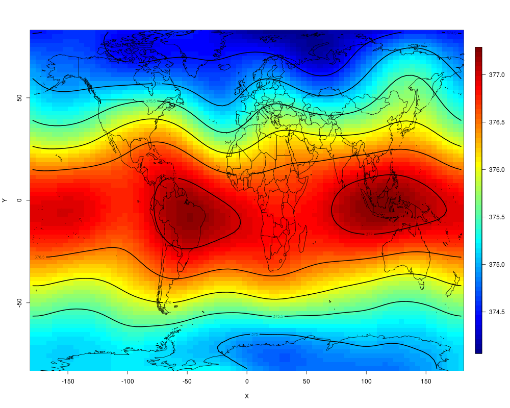
# fit the CO2 satellite data with a fixed lambda
# (use a very small number of basis functions so example
#  runs quickly)
 data(CO2)
  LKinfo1<- LKrigSetup(CO2$lon.lat, NC=8 ,nlevel=1, lambda=.2,
                       a.wght=5, alpha=1, 
                       LKGeometry="LKRing" )                                         
  obj1<- LKrig( CO2$lon.lat,CO2$y,LKinfo=LKinfo1)	
# take a look: 
surface( obj1)
world( add=TRUE)  
# compare to fitting without wrapping
#  LKinfo2<- LKrigSetup(CO2$lon.lat, NC=8 ,nlevel=1,
#                   lambda=.2, a.wght=5, alpha=1 )                                         
#  obj2<- LKrig( CO2$lon.lat,CO2$y,LKinfo=LKinfo2)	
# not periodic in longitude:
# surface(obj2)  

Results

R version 3.3.1 (2016-06-21) -- "Bug in Your Hair"
Copyright (C) 2016 The R Foundation for Statistical Computing
Platform: x86_64-pc-linux-gnu (64-bit)

R is free software and comes with ABSOLUTELY NO WARRANTY.
You are welcome to redistribute it under certain conditions.
Type 'license()' or 'licence()' for distribution details.

R is a collaborative project with many contributors.
Type 'contributors()' for more information and
'citation()' on how to cite R or R packages in publications.

Type 'demo()' for some demos, 'help()' for on-line help, or
'help.start()' for an HTML browser interface to help.
Type 'q()' to quit R.

> library(LatticeKrig)
Loading required package: spam
Loading required package: grid
Spam version 1.3-0 (2015-10-24) is loaded.
Type 'help( Spam)' or 'demo( spam)' for a short introduction 
and overview of this package.
Help for individual functions is also obtained by adding the
suffix '.spam' to the function name, e.g. 'help( chol.spam)'.

Attaching package: 'spam'

The following objects are masked from 'package:base':

    backsolve, forwardsolve

Loading required package: fields
Loading required package: maps

 # maps v3.1: updated 'world': all lakes moved to separate new #
 # 'lakes' database. Type '?world' or 'news(package="maps")'.  #


> png(filename="/home/ddbj/snapshot/RGM3/R_CC/result/LatticeKrig/PeriodicGeometry.Rd_%03d_medium.png", width=480, height=480)
> ### Name: Periodic geometries for  spherical data. 
> ### Title: Geometries to approximate a cross section of 2-d and 3-d
> ###   spherical data.
> ### Aliases: LKRing LKCylinder
> ### Keywords: spatial
> 
> ### ** Examples
> 
> # 	
> # fit the CO2 satellite data with a fixed lambda
> # (use a very small number of basis functions so example
> #  runs quickly)
>  data(CO2)
>   LKinfo1<- LKrigSetup(CO2$lon.lat, NC=8 ,nlevel=1, lambda=.2,
+                        a.wght=5, alpha=1, 
+                        LKGeometry="LKRing" )                                         
>   obj1<- LKrig( CO2$lon.lat,CO2$y,LKinfo=LKinfo1)	
> # take a look: 
> surface( obj1)
> world( add=TRUE)  
> # compare to fitting without wrapping
> #  LKinfo2<- LKrigSetup(CO2$lon.lat, NC=8 ,nlevel=1,
> #                   lambda=.2, a.wght=5, alpha=1 )                                         
> #  obj2<- LKrig( CO2$lon.lat,CO2$y,LKinfo=LKinfo2)	
> # not periodic in longitude:
> # surface(obj2)  
> 
> 
> 
> 
> 
> 
> dev.off()
null device 
          1 
>