Linearized Bregman solver for composite conditionally likelihood of Ising model with lasso penalty.

Description

Solver for the entire solution path of coefficients.

Usage

ising(X, kappa, alpha, c = 2, tlist, responses = c(-1, 1), nt = 100,
  trate = 100, intercept = TRUE, print = FALSE)

Arguments

Details

The data matrix X is assumed in {1,-1}. The Ising model here used is described as following:

P(x) sim exp(∑_i frac{a_{0i}}{2}x_i + x^T Θ x/4)

where Θ is p-by-p symmetric and 0 on diagnal. Then conditional on x_{-j}

frac{P(x_j=1)}{P(x_j=-1)} = exp(∑_i a_{0i} + ∑_{i\neq j}θ_{ji}x_i)

then the composite conditional likelihood is like this:

- ∑_{j} condloglik(X_j | X_{-j})

Value

A "ising" class object is returned. The list contains the call, the path, the intercept term a0 and value for alpha, kappa, t.

Author(s)

Jiechao Xiong

Examples

library('Libra')
library('igraph')
data('west10')
X <- as.matrix(2*west10-1);
obj = ising(X,10,0.1,nt=1000,trate=100)
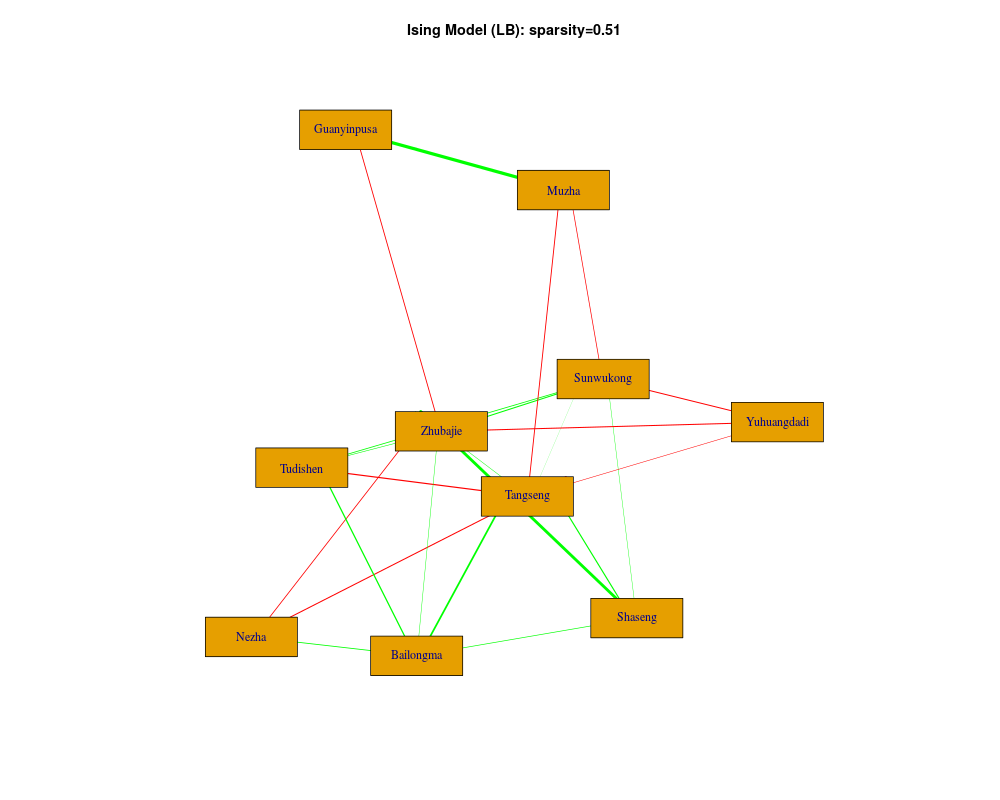
g<-graph.adjacency(obj$path[,,770],mode="undirected",weighted=TRUE)
E(g)[E(g)$weight<0]$color<-"red"
E(g)[E(g)$weight>0]$color<-"green"
V(g)$name<-attributes(west10)$names
plot(g,vertex.shape="rectangle",vertex.size=35,vertex.label=V(g)$name,
edge.width=2*abs(E(g)$weight),main="Ising Model (LB): sparsity=0.51")

Results

R version 3.3.1 (2016-06-21) -- "Bug in Your Hair"
Copyright (C) 2016 The R Foundation for Statistical Computing
Platform: x86_64-pc-linux-gnu (64-bit)

R is free software and comes with ABSOLUTELY NO WARRANTY.
You are welcome to redistribute it under certain conditions.
Type 'license()' or 'licence()' for distribution details.

R is a collaborative project with many contributors.
Type 'contributors()' for more information and
'citation()' on how to cite R or R packages in publications.

Type 'demo()' for some demos, 'help()' for on-line help, or
'help.start()' for an HTML browser interface to help.
Type 'q()' to quit R.

> library(Libra)
Loading required package: nnls
Loaded Libra 1.5

> png(filename="/home/ddbj/snapshot/RGM3/R_CC/result/Libra/ising.Rd_%03d_medium.png", width=480, height=480)
> ### Name: ising
> ### Title: Linearized Bregman solver for composite conditionally likelihood
> ###   of Ising model with lasso penalty.
> ### Aliases: ising
> ### Keywords: regression
> 
> ### ** Examples
> 
> 
> library('Libra')
> library('igraph')

Attaching package: 'igraph'

The following objects are masked from 'package:stats':

    decompose, spectrum

The following object is masked from 'package:base':

    union

> data('west10')
> X <- as.matrix(2*west10-1);
> obj = ising(X,10,0.1,nt=1000,trate=100)
> g<-graph.adjacency(obj$path[,,770],mode="undirected",weighted=TRUE)
> E(g)[E(g)$weight<0]$color<-"red"
> E(g)[E(g)$weight>0]$color<-"green"
> V(g)$name<-attributes(west10)$names
> plot(g,vertex.shape="rectangle",vertex.size=35,vertex.label=V(g)$name,
+ edge.width=2*abs(E(g)$weight),main="Ising Model (LB): sparsity=0.51")
> 
> 
> 
> 
> 
> dev.off()
null device 
          1 
>