Extended Power Lindley Distribution

Description

Density function, distribution function, quantile function, random number generation and hazard rate function for the extended power Lindley distribution with parameters theta, alpha and beta.

Usage

dextplindley(x, theta, alpha, beta, log = FALSE)

pextplindley(q, theta, alpha, beta, lower.tail = TRUE, log.p = FALSE)

qextplindley(p, theta, alpha, beta, lower.tail = TRUE, log.p = FALSE)

rextplindley(n, theta, alpha, beta, mixture = TRUE)

hextplindley(x, theta, alpha, beta, log = FALSE)

Arguments

Details

Probability density function

f(xmid θ,α,β )={frac{α θ ^{2}}{θ +β }}(1+β x^{α }) x^{α -1} e^{-θ x^{α }}

Cumulative distribution function

F(xmid θ,α,β )=1-≤ft( 1+{frac{β θ x^{α }}{θ +β }} ight) e^{-θ x^{α }}

Quantile function

Q(pmid θ ,α ,β )={≤ft[ -frac{1}{θ }-frac{1}{β }-{frac{1}{θ }}W_{-1}{≤ft( frac{1}{β }≤ft( p-1 ight) ≤ft( β +θ ight) e{{^{-≤ft( {frac{β +θ }{β }} ight) }}} ight) } ight] }^{frac{1}{α }}

Hazard rate function

h(xmid θ ,α ,β )={frac{α {θ }^{2}≤ft( 1+β {x}^{α } ight) {x}^{α -1}}{≤ft( β +θ ight) {≤ft(1+{frac{β θ {x}^{α }}{β +θ }} ight) }}}

where W_{-1} denotes the negative branch of the Lambert W function.

Particular cases: β = 1 the power Lindley distribution, α = 1 the two-parameter Lindley distribution and (α = 1, β = 1) the one-parameter Lindley distribution.

Value

dextplindley gives the density, pextplindley gives the distribution function, qextplindley gives the quantile function, rextplindley generates random deviates and hextplindley gives the hazard rate function.

Invalid arguments will return an error message.

Author(s)

Josmar Mazucheli jmazucheli@gmail.com

Larissa B. Fernandes lbf.estatistica@gmail.com

Source

[d-h-p-q-r]extplindley are calculated directly from the definitions. rextplindley uses either a two-component mixture of gamma distributions or the quantile function.

References

Alkarni, S. H., (2015). Extended power Lindley distribution: A new statistical model for non-monotone survival data. European Journal of Statistics and Probability, 3, (3), 19-34.

See Also

lambertWm1.

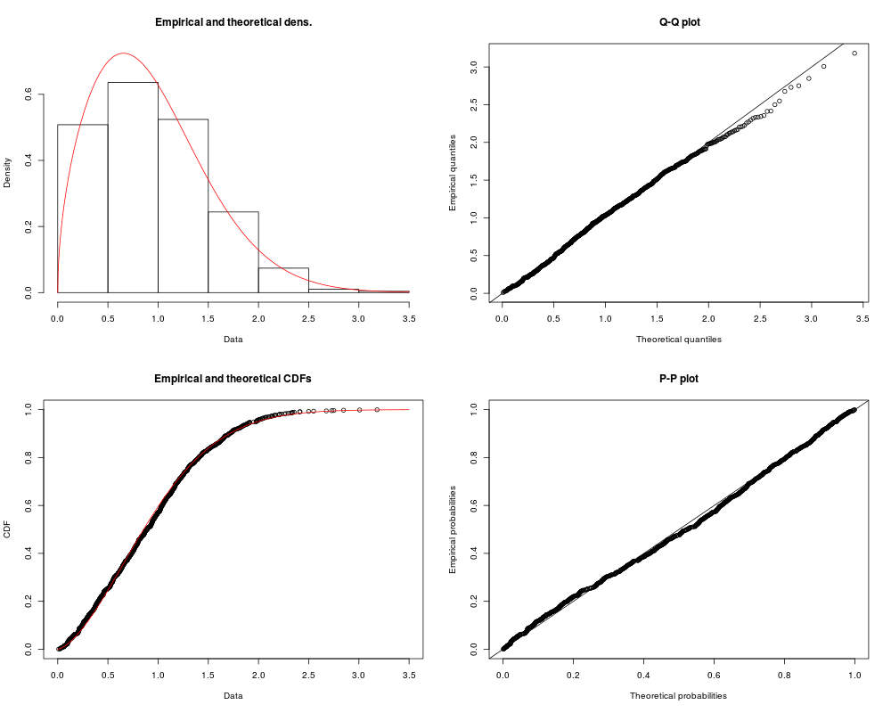
Examples

set.seed(1)
x <- rextplindley(n = 1000, theta = 1.5, alpha = 1.5, beta = 1.5, mixture = TRUE)
R <- range(x)
S <- seq(from = R[1], to = R[2], by = 0.1)
plot(S, dextplindley(S, theta = 1.5, alpha = 1.5, beta = 1.5), xlab = 'x', ylab = 'pdf')
hist(x, prob = TRUE, main = '', add = TRUE)

p <- seq(from = 0.1, to = 0.9, by = 0.1)
q <- quantile(x, prob = p)
pextplindley(q, theta = 1.5, alpha = 1.5, beta = 1.5, lower.tail = TRUE)
pextplindley(q, theta = 1.5, alpha = 1.5, beta = 1.5, lower.tail = FALSE)
qextplindley(p, theta = 1.5, alpha = 1.5, beta = 1.5, lower.tail = TRUE)
qextplindley(p, theta = 1.5, alpha = 1.5, beta = 1.5, lower.tail = FALSE)

library(fitdistrplus)
fit <- fitdist(x, 'extplindley', start = list(theta = 1.5, alpha = 1.5, beta = 1.5))
plot(fit)

Results

R version 3.3.1 (2016-06-21) -- "Bug in Your Hair"
Copyright (C) 2016 The R Foundation for Statistical Computing
Platform: x86_64-pc-linux-gnu (64-bit)

R is free software and comes with ABSOLUTELY NO WARRANTY.
You are welcome to redistribute it under certain conditions.
Type 'license()' or 'licence()' for distribution details.

R is a collaborative project with many contributors.
Type 'contributors()' for more information and
'citation()' on how to cite R or R packages in publications.

Type 'demo()' for some demos, 'help()' for on-line help, or
'help.start()' for an HTML browser interface to help.
Type 'q()' to quit R.

> library(LindleyR)
> png(filename="/home/ddbj/snapshot/RGM3/R_CC/result/LindleyR/EXTPLindley.Rd_%03d_medium.png", width=480, height=480)
> ### Name: EXTPLindley
> ### Title: Extended Power Lindley Distribution
> ### Aliases: EXTPLindley dextplindley hextplindley pextplindley
> ###   qextplindley rextplindley
> 
> ### ** Examples
> 
> set.seed(1)
> x <- rextplindley(n = 1000, theta = 1.5, alpha = 1.5, beta = 1.5, mixture = TRUE)
> R <- range(x)
> S <- seq(from = R[1], to = R[2], by = 0.1)
> plot(S, dextplindley(S, theta = 1.5, alpha = 1.5, beta = 1.5), xlab = 'x', ylab = 'pdf')
> hist(x, prob = TRUE, main = '', add = TRUE)
> 
> p <- seq(from = 0.1, to = 0.9, by = 0.1)
> q <- quantile(x, prob = p)
> pextplindley(q, theta = 1.5, alpha = 1.5, beta = 1.5, lower.tail = TRUE)
       10%        20%        30%        40%        50%        60%        70% 
0.09043284 0.19088343 0.30270800 0.42976695 0.53676346 0.63408851 0.72294224 
       80%        90% 
0.81556374 0.90557336 
> pextplindley(q, theta = 1.5, alpha = 1.5, beta = 1.5, lower.tail = FALSE)
       10%        20%        30%        40%        50%        60%        70% 
0.90956716 0.80911657 0.69729200 0.57023305 0.46323654 0.36591149 0.27705776 
       80%        90% 
0.18443626 0.09442664 
> qextplindley(p, theta = 1.5, alpha = 1.5, beta = 1.5, lower.tail = TRUE)
[1] 0.2620596 0.4207329 0.5613218 0.6971077 0.8358167 0.9849223 1.1550334
[8] 1.3669455 1.6818918
> qextplindley(p, theta = 1.5, alpha = 1.5, beta = 1.5, lower.tail = FALSE)
[1] 1.6818918 1.3669455 1.1550334 0.9849223 0.8358167 0.6971077 0.5613218
[8] 0.4207329 0.2620596
> 
> library(fitdistrplus)
Loading required package: MASS
> fit <- fitdist(x, 'extplindley', start = list(theta = 1.5, alpha = 1.5, beta = 1.5))
> plot(fit)
> 
> 
> 
> 
> 
> 
> dev.off()
null device 
          1 
>