R Graphical Manual

Browse All

Last data update: 2014.03.03

R: Transform a CW-OSL curve into a pHM-OSL curve via...

CW2pHMi

R Documentation

Transform a CW-OSL curve into a pHM-OSL curve via interpolation under hyperbolic modulation conditions

Description

This function transforms a conventionally measured continuous-wave (CW) OSL-curve to a pseudo hyperbolic modulated (pHM) curve under hyperbolic modulation conditions using the interpolation procedure described by Bos & Wallinga (2012).

Usage

CW2pHMi(values, delta)

Arguments

`values`	`RLum.Data.Curve` or `data.frame` (required): `RLum.Data.Curve` or `data.frame` with measured curve data of type stimulation time (t) (`values[,1]`) and measured counts (cts) (`values[,2]`).
`delta`	`vector` (optional): stimulation rate parameter, if no value is given, the optimal value is estimated automatically (see details). Smaller values of delta produce more points in the rising tail of the curve.

Details

The complete procedure of the transformation is described in Bos & Wallinga (2012). The input data.frame consists of two columns: time (t) and count values (CW(t))

Internal transformation steps

(1) log(CW-OSL) values

(2) Calculate t' which is the transformed time:

t' = t-(1/δ)*log(1+δ*t)

(3) Interpolate CW(t'), i.e. use the log(CW(t)) to obtain the count values for the transformed time (t'). Values beyond min(t) and max(t) produce NA values.

(4) Select all values for t' < min(t), i.e. values beyond the time resolution of t. Select the first two values of the transformed data set which contain no NA values and use these values for a linear fit using lm.

(5) Extrapolate values for t' < min(t) based on the previously obtained fit parameters.

(6) Transform values using

pHM(t) = (δ*t/(1+δ*t))*c*CW(t')

c = (1+δ*P)/δ*P

P = length(stimulation~period)

(7) Combine all values and truncate all values for t' > max(t)

The number of values for t' < min(t) depends on the stimulation rate parameter delta. To avoid the production of too many artificial data at the raising tail of the determined pHM curve, it is recommended to use the automatic estimation routine for delta, i.e. provide no value for delta.

Value

The function returns the same data type as the input data type with the transformed curve values.

list(list("RLum.Data.Curve"))

package RLum object with two additional info elements:

$CW2pHMi.x.t	: transformed time values
$CW2pHMi.method	: used method for the production of the new data points

list(list("data.frame"))

with four columns:

$x	: time
$y.t	: transformed count values
$x.t	: transformed time values
$method	: used method for the production of the new data points

Function version

0.2.2 (2015-11-29 17:27:48)

Note

According to Bos & Wallinga (2012), the number of extrapolated points should be limited to avoid artificial intensity data. If delta is provided manually and more than two points are extrapolated, a warning message is returned.

The function approx may produce some Inf and NaN data. The function tries to manually interpolate these values by calculating the mean using the adjacent channels. If two invalid values are succeeding, the values are removed and no further interpolation is attempted.
In every case a warning message is shown.

Author(s)

Sebastian Kreutzer, IRAMAT-CRP2A, Universite Bordeaux Montaigne (France)

Based on comments and suggestions from:
Adrie J.J. Bos, Delft University of Technology, The Netherlands

R Luminescence Package Team

References

Bos, A.J.J. & Wallinga, J., 2012. How to visualize quartz OSL signal components. Radiation Measurements, 47, 752-758.

Further Reading

Bulur, E., 1996. An Alternative Technique For Optically Stimulated Luminescence (OSL) Experiment. Radiation Measurements, 26, 701-709.

Bulur, E., 2000. A simple transformation for converting CW-OSL curves to LM-OSL curves. Radiation Measurements, 32, 141-145.

Examples



##(1) - simple transformation

##load CW-OSL curve data
data(ExampleData.CW_OSL_Curve, envir = environment())

##transform values
values.transformed<-CW2pHMi(ExampleData.CW_OSL_Curve)

##plot
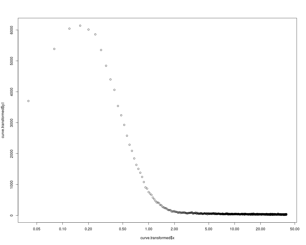
plot(values.transformed$x, values.transformed$y.t, log = "x")

##(2) - load CW-OSL curve from BIN-file and plot transformed values

##load BINfile
#BINfileData<-readBIN2R("[path to BIN-file]")
data(ExampleData.BINfileData, envir = environment())

##grep first CW-OSL curve from ALQ 1
curve.ID<-CWOSL.SAR.Data@METADATA[CWOSL.SAR.Data@METADATA[,"LTYPE"]=="OSL" &
                                    CWOSL.SAR.Data@METADATA[,"POSITION"]==1
                                  ,"ID"]

curve.HIGH<-CWOSL.SAR.Data@METADATA[CWOSL.SAR.Data@METADATA[,"ID"]==curve.ID[1]
                                    ,"HIGH"]

curve.NPOINTS<-CWOSL.SAR.Data@METADATA[CWOSL.SAR.Data@METADATA[,"ID"]==curve.ID[1]
                                       ,"NPOINTS"]

##combine curve to data set

curve<-data.frame(x = seq(curve.HIGH/curve.NPOINTS,curve.HIGH,
                          by = curve.HIGH/curve.NPOINTS),
                  y=unlist(CWOSL.SAR.Data@DATA[curve.ID[1]]))


##transform values

curve.transformed <- CW2pHMi(curve)

##plot curve
plot(curve.transformed$x, curve.transformed$y.t, log = "x")


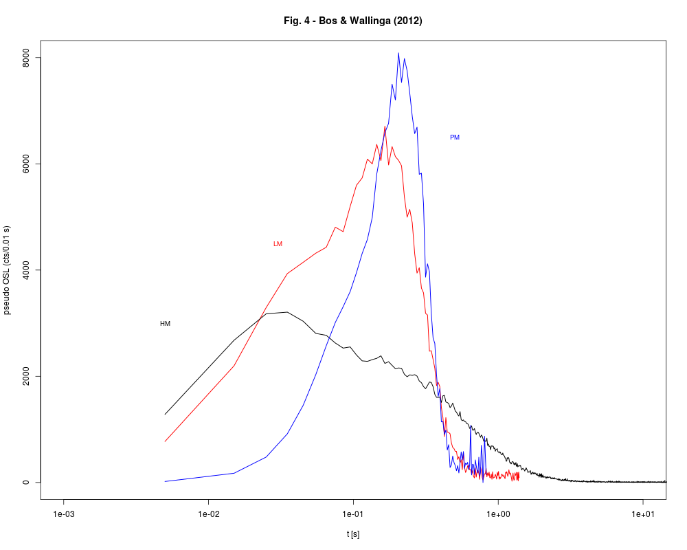
##(3) - produce Fig. 4 from Bos & Wallinga (2012)

##load data
data(ExampleData.CW_OSL_Curve, envir = environment())
values <- CW_Curve.BosWallinga2012

##open plot area
plot(NA, NA,
     xlim=c(0.001,10),
     ylim=c(0,8000),
     ylab="pseudo OSL (cts/0.01 s)",
     xlab="t [s]",
     log="x",
     main="Fig. 4 - Bos & Wallinga (2012)")

values.t<-CW2pLMi(values, P=1/20)
lines(values[1:length(values.t[,1]),1],CW2pLMi(values, P=1/20)[,2],
      col="red" ,lwd=1.3)
text(0.03,4500,"LM", col="red" ,cex=.8)

values.t<-CW2pHMi(values, delta=40)
lines(values[1:length(values.t[,1]),1],CW2pHMi(values, delta=40)[,2],
      col="black", lwd=1.3)
text(0.005,3000,"HM", cex=.8)

values.t<-CW2pPMi(values, P=1/10)
lines(values[1:length(values.t[,1]),1],CW2pPMi(values, P=1/10)[,2],
      col="blue", lwd=1.3)
text(0.5,6500,"PM", col="blue" ,cex=.8)

Results


R version 3.3.1 (2016-06-21) -- "Bug in Your Hair"
Copyright (C) 2016 The R Foundation for Statistical Computing
Platform: x86_64-pc-linux-gnu (64-bit)

R is free software and comes with ABSOLUTELY NO WARRANTY.
You are welcome to redistribute it under certain conditions.
Type 'license()' or 'licence()' for distribution details.

R is a collaborative project with many contributors.
Type 'contributors()' for more information and
'citation()' on how to cite R or R packages in publications.

Type 'demo()' for some demos, 'help()' for on-line help, or
'help.start()' for an HTML browser interface to help.
Type 'q()' to quit R.

> library(Luminescence)
Welcome to the R package Luminescence version 0.6.0 [Built: 2016-05-30 16:47:30 UTC]
The true age: 'How many roads...'
> png(filename="/home/ddbj/snapshot/RGM3/R_CC/result/Luminescence/CW2pHMi.Rd_%03d_medium.png", width=480, height=480)
> ### Name: CW2pHMi
> ### Title: Transform a CW-OSL curve into a pHM-OSL curve via interpolation
> ###   under hyperbolic modulation conditions
> ### Aliases: CW2pHMi
> ### Keywords: manip
> 
> ### ** Examples
> 
> 
> 
> ##(1) - simple transformation
> 
> ##load CW-OSL curve data
> data(ExampleData.CW_OSL_Curve, envir = environment())
> 
> ##transform values
> values.transformed<-CW2pHMi(ExampleData.CW_OSL_Curve)
> 
> ##plot
> plot(values.transformed$x, values.transformed$y.t, log = "x")
> 
> ##(2) - load CW-OSL curve from BIN-file and plot transformed values
> 
> ##load BINfile
> #BINfileData<-readBIN2R("[path to BIN-file]")
> data(ExampleData.BINfileData, envir = environment())
> 
> ##grep first CW-OSL curve from ALQ 1
> curve.ID<-CWOSL.SAR.Data@METADATA[CWOSL.SAR.Data@METADATA[,"LTYPE"]=="OSL" &
+                                     CWOSL.SAR.Data@METADATA[,"POSITION"]==1
+                                   ,"ID"]
> 
> curve.HIGH<-CWOSL.SAR.Data@METADATA[CWOSL.SAR.Data@METADATA[,"ID"]==curve.ID[1]
+                                     ,"HIGH"]
> 
> curve.NPOINTS<-CWOSL.SAR.Data@METADATA[CWOSL.SAR.Data@METADATA[,"ID"]==curve.ID[1]
+                                        ,"NPOINTS"]
> 
> ##combine curve to data set
> 
> curve<-data.frame(x = seq(curve.HIGH/curve.NPOINTS,curve.HIGH,
+                           by = curve.HIGH/curve.NPOINTS),
+                   y=unlist(CWOSL.SAR.Data@DATA[curve.ID[1]]))
> 
> 
> ##transform values
> 
> curve.transformed <- CW2pHMi(curve)
> 
> ##plot curve
> plot(curve.transformed$x, curve.transformed$y.t, log = "x")
> 
> 
> ##(3) - produce Fig. 4 from Bos & Wallinga (2012)
> 
> ##load data
> data(ExampleData.CW_OSL_Curve, envir = environment())
> values <- CW_Curve.BosWallinga2012
> 
> ##open plot area
> plot(NA, NA,
+      xlim=c(0.001,10),
+      ylim=c(0,8000),
+      ylab="pseudo OSL (cts/0.01 s)",
+      xlab="t [s]",
+      log="x",
+      main="Fig. 4 - Bos & Wallinga (2012)")
> 
> values.t<-CW2pLMi(values, P=1/20)
> lines(values[1:length(values.t[,1]),1],CW2pLMi(values, P=1/20)[,2],
+       col="red" ,lwd=1.3)
> text(0.03,4500,"LM", col="red" ,cex=.8)
> 
> values.t<-CW2pHMi(values, delta=40)
Warning message:
In CW2pHMi(values, delta = 40) :
  56  values have been found and replaced the mean of the nearest values.
> lines(values[1:length(values.t[,1]),1],CW2pHMi(values, delta=40)[,2],
+       col="black", lwd=1.3)
Warning message:
In CW2pHMi(values, delta = 40) :
  56  values have been found and replaced the mean of the nearest values.
> text(0.005,3000,"HM", cex=.8)
> 
> values.t<-CW2pPMi(values, P=1/10)
Warning message:
In CW2pPMi(values, P = 1/10) :
  t' is beyond the time resolution. Only two data points have been extrapolated, the first 3 points have been set to 0!
> lines(values[1:length(values.t[,1]),1],CW2pPMi(values, P=1/10)[,2],
+       col="blue", lwd=1.3)
Warning message:
In CW2pPMi(values, P = 1/10) :
  t' is beyond the time resolution. Only two data points have been extrapolated, the first 3 points have been set to 0!
> text(0.5,6500,"PM", col="blue" ,cex=.8)
> 
> 
> 
> 
> 
> 
> 
> dev.off()
null device 
          1 
>