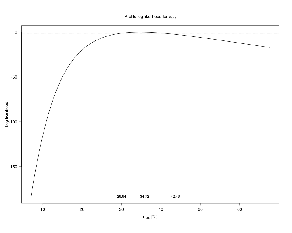
Apply the central age model (CAM) after Galbraith et al. (1999) to a given De distribution

Description

This function calculates the central dose and dispersion of the De distribution, their standard errors and the profile log likelihood function for sigma.

Usage

calc_CentralDose(data, sigmab, log = TRUE, plot = TRUE, ...)

Arguments

Details

This function uses the equations of Galbraith & Roberts (2012). The parameters delta and sigma are estimated by numerically solving eq. 15 and 16. Their standard errors are approximated using eq. 17. In addition, the profile log-likelihood function for sigma is calculated using eq. 18 and presented as a plot. Numerical values of the maximum likelihood approach are only presented in the plot and not in the console. A detailed explanation on maximum likelihood estimation can be found in the appendix of Galbraith & Laslett (1993, 468-470) and Galbraith & Roberts (2012, 15)

Value

Returns a plot (optional) and terminal output. In addition an RLum.Results object is returned containing the following element:

The output should be accessed using the function get_RLum

Function version

1.3.1 (2016-05-02 09:36:06)

Author(s)

Christoph Burow, University of Cologne (Germany)
Based on a rewritten S script of Rex Galbraith, 2010

R Luminescence Package Team

References

Galbraith, R.F. & Laslett, G.M., 1993. Statistical models for mixed fission track ages. Nuclear Tracks Radiation Measurements 4, 459-470.

Galbraith, R.F., Roberts, R.G., Laslett, G.M., Yoshida, H. & Olley, J.M., 1999. Optical dating of single grains of quartz from Jinmium rock shelter, northern Australia. Part I: experimental design and statistical models. Archaeometry 41, 339-364.

Galbraith, R.F. & Roberts, R.G., 2012. Statistical aspects of equivalent dose and error calculation and display in OSL dating: An overview and some recommendations. Quaternary Geochronology 11, 1-27.

Further reading

Arnold, L.J. & Roberts, R.G., 2009. Stochastic modelling of multi-grain equivalent dose (De) distributions: Implications for OSL dating of sediment mixtures. Quaternary Geochronology 4, 204-230.

Bailey, R.M. & Arnold, L.J., 2006. Statistical modelling of single grain quartz De distributions and an assessment of procedures for estimating burial dose. Quaternary Science Reviews 25, 2475-2502.

Cunningham, A.C. & Wallinga, J., 2012. Realizing the potential of fluvial archives using robust OSL chronologies. Quaternary Geochronology 12, 98-106.

Rodnight, H., Duller, G.A.T., Wintle, A.G. & Tooth, S., 2006. Assessing the reproducibility and accuracy of optical dating of fluvial deposits. Quaternary Geochronology, 1 109-120.

Rodnight, H., 2008. How many equivalent dose values are needed to obtain a reproducible distribution?. Ancient TL 26, 3-10.

See Also

plot, calc_CommonDose, calc_FiniteMixture, calc_FuchsLang2001, calc_MinDose

Examples

##load example data
data(ExampleData.DeValues, envir = environment())

##apply the central dose model
calc_CentralDose(ExampleData.DeValues$CA1)

Results

R version 3.3.1 (2016-06-21) -- "Bug in Your Hair"
Copyright (C) 2016 The R Foundation for Statistical Computing
Platform: x86_64-pc-linux-gnu (64-bit)

R is free software and comes with ABSOLUTELY NO WARRANTY.
You are welcome to redistribute it under certain conditions.
Type 'license()' or 'licence()' for distribution details.

R is a collaborative project with many contributors.
Type 'contributors()' for more information and
'citation()' on how to cite R or R packages in publications.

Type 'demo()' for some demos, 'help()' for on-line help, or
'help.start()' for an HTML browser interface to help.
Type 'q()' to quit R.

> library(Luminescence)
Welcome to the R package Luminescence version 0.6.0 [Built: 2016-05-30 16:47:30 UTC]
A Windows user: 'An apple a day keeps the doctor away.'
> png(filename="/home/ddbj/snapshot/RGM3/R_CC/result/Luminescence/calc_CentralDose.Rd_%03d_medium.png", width=480, height=480)
> ### Name: calc_CentralDose
> ### Title: Apply the central age model (CAM) after Galbraith et al. (1999)
> ###   to a given De distribution
> ### Aliases: calc_CentralDose
> 
> ### ** Examples
> 
> 
> ##load example data
> data(ExampleData.DeValues, envir = environment())
> 
> ##apply the central dose model
> calc_CentralDose(ExampleData.DeValues$CA1)

 [calc_CentralDose]

----------- meta data ----------------
 n:                       62
 log:                     TRUE
----------- dose estimate ------------
 central dose [Gy]:       65.71
 SE [Gy]:                 3.05
 rel. SE [%]:             4.65
----------- overdispersion -----------
 OD [Gy]:                 22.79
 SE [Gy]:                 2.27
 OD [%]:                  34.69
 SE [%]:                  3.46
-------------------------------------

> 
> 
> 
> 
> 
> 
> dev.off()
null device 
          1 
>