R: Apply the maximum age model to a given De distribution
calc_MaxDose
R Documentation
Apply the maximum age model to a given De distribution
Description
Function to fit the maximum age model to De data. This is a wrapper function
that calls calc_MinDose() and applies a similiar approach as described in
Olley et al. (2006).
RLum.Results or data.frame
(required): for data.frame: two columns with De
(data[,1]) and De error (values[,2])
sigmab
numeric (required): spread in De values
given as a fraction (e.g. 0.2). This value represents the expected
overdispersion in the data should the sample be well-bleached (Cunningham &
Walling 2012, p. 100).
log
logical (with default): fit the (un-)logged three
parameter minimum dose model to De data
par
numeric (with default): apply the 3- or
4-parametric minimum age model (par=3 or par=4).
bootstrap
logical (with default): apply the recycled
bootstrap approach of Cunningham & Wallinga (2012).
init.values
numeric (with default): starting values for
gamma, sigma, p0 and mu. Custom values need to be provided in a vector of
length three in the form of c(gamma, sigma, p0).
plot
logical (with default): plot output
(TRUE/FALSE)
...
further arguments for bootstrapping (bs.M, bs.N, bs.h,
sigmab.sd). See details for their usage.
Details
Data transformation
To estimate the maximum dose population
and its standard error, the three parameter minimum age model of Galbraith
et al. (1999) is adapted. The measured De values are transformed as follows:
1. convert De values to natural logs 2. multiply the logged data
to creat a mirror image of the De distribution 3. shift De values along
x-axis by the smallest x-value found to obtain only positive values 4.
combine in quadrature the measurement error associated with each De value
with a relative error specified by sigmab 5. apply the MAM to these data
When all calculations are done the results are then converted as
follows
1. subtract the x-offset 2. multiply the natural logs by
-1 3. take the exponent to obtain the maximum dose estimate in Gy
Further documentation
Please see calc_MinDose.
Value
Please see calc_MinDose.
Function version
0.3 (2015-11-29 17:27:48)
Author(s)
Christoph Burow, University of Cologne (Germany) Based on a
rewritten S script of Rex Galbraith, 2010
R Luminescence Package Team
References
Arnold, L.J., Roberts, R.G., Galbraith, R.F. & DeLong, S.B.,
2009. A revised burial dose estimation procedure for optical dating of young
and modern-age sediments. Quaternary Geochronology 4, 306-325.
Galbraith, R.F., Roberts, R.G., Laslett, G.M., Yoshida, H. & Olley, J.M.,
1999. Optical dating of single grains of quartz from Jinmium rock shelter,
northern Australia. Part I: experimental design and statistical models.
Archaeometry 41, 339-364.
Galbraith,
R.F. & Roberts, R.G., 2012. Statistical aspects of equivalent dose and error
calculation and display in OSL dating: An overview and some recommendations.
Quaternary Geochronology 11, 1-27.
Olley, J.M., Roberts, R.G.,
Yoshida, H., Bowler, J.M., 2006. Single-grain optical dating of grave-infill
associated with human burials at Lake Mungo, Australia. Quaternary Science
Reviews 25, 2469-2474.
Further reading
Arnold, L.J. &
Roberts, R.G., 2009. Stochastic modelling of multi-grain equivalent dose
(De) distributions: Implications for OSL dating of sediment mixtures.
Quaternary Geochronology 4, 204-230.
Bailey, R.M. & Arnold, L.J.,
2006. Statistical modelling of single grain quartz De distributions and an
assessment of procedures for estimating burial dose. Quaternary Science
Reviews 25, 2475-2502.
Cunningham, A.C. & Wallinga, J., 2012.
Realizing the potential of fluvial archives using robust OSL chronologies.
Quaternary Geochronology 12, 98-106.
Rodnight, H., Duller, G.A.T.,
Wintle, A.G. & Tooth, S., 2006. Assessing the reproducibility and accuracy
of optical dating of fluvial deposits. Quaternary Geochronology 1, 109-120.
Rodnight, H., 2008. How many equivalent dose values are needed to
obtain a reproducible distribution?. Ancient TL 26, 3-10.
## load example data
data(ExampleData.DeValues, envir = environment())

# apply the maximum dose model
calc_MaxDose(ExampleData.DeValues$CA1, sigmab = 0.2, par = 3)
Results
R version 3.3.1 (2016-06-21) -- "Bug in Your Hair"
Copyright (C) 2016 The R Foundation for Statistical Computing
Platform: x86_64-pc-linux-gnu (64-bit)
R is free software and comes with ABSOLUTELY NO WARRANTY.
You are welcome to redistribute it under certain conditions.
Type 'license()' or 'licence()' for distribution details.
R is a collaborative project with many contributors.
Type 'contributors()' for more information and
'citation()' on how to cite R or R packages in publications.
Type 'demo()' for some demos, 'help()' for on-line help, or
'help.start()' for an HTML browser interface to help.
Type 'q()' to quit R.
> library(Luminescence)
Welcome to the R package Luminescence version 0.6.0 [Built: 2016-05-30 16:47:30 UTC]
A tunnelling electron: 'God does not play dice.'
> png(filename="/home/ddbj/snapshot/RGM3/R_CC/result/Luminescence/calc_MaxDose.Rd_%03d_medium.png", width=480, height=480)
> ### Name: calc_MaxDose
> ### Title: Apply the maximum age model to a given De distribution
> ### Aliases: calc_MaxDose
>
> ### ** Examples
>
>
> ## load example data
> data(ExampleData.DeValues, envir = environment())
>
> # apply the maximum dose model
> calc_MaxDose(ExampleData.DeValues$CA1, sigmab = 0.2, par = 3)
----------- meta data -----------
n par sigmab logged Lmax BIC
62 3 0.2 TRUE -19.79245 58.86603
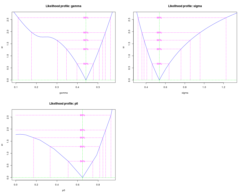
--- final parameter estimates ---
gamma sigma p0 mu
4.34 0.54 0.65 0
------ confidence intervals -----
2.5 % 97.5 %
gamma 4.24 4.60
sigma 0.36 0.96
p0 NA 0.87
------ De (asymmetric error) -----
De lower upper
76.58 1.2 1.71
------ De (symmetric error) -----
De error
76.58 7.57
>
>
>
>
>
>
> dev.off()
null device
1
>
 .
.