Apply the (un-)logged minimum age model (MAM) after Galbraith et al. (1999) to a given De distribution

Description

Function to fit the (un-)logged three or four parameter minimum dose model (MAM-3/4) to De data.

Usage

calc_MinDose(data, sigmab, log = TRUE, par = 3, bootstrap = FALSE,
  init.values, level = 0.95, plot = TRUE, multicore = FALSE, ...)

Arguments

Details

Parameters

This model has four parameters:

If par=3 (default) the 3-parametric minimum age model is applied, where gamma=mu. For par=4 the 4-parametric model is applied instead.

(Un-)logged model

In the original version of the three-parameter minimum dose model, the basic data are the natural logarithms of the De estimates and relative standard errors of the De estimates. This model will be applied if log=TRUE.

If log=FALSE, the modified un-logged model will be applied instead. This has essentially the same form as the original version. gamma and sigma are in Gy and gamma becomes the minimum true dose in the population.

While the original (logged) version of the mimimum dose model may be appropriate for most samples (i.e. De distributions), the modified (un-logged) version is specially designed for modern-age and young samples containing negative, zero or near-zero De estimates (Arnold et al. 2009, p. 323).

Initial values & boundaries

The log likelihood calculations use the nlminb function for box-constrained optimisation using PORT routines. Accordingly, initial values for the four parameters can be specified via init.values. If no values are provided for init.values reasonable starting values are estimated from the input data. If the final estimates of gamma, mu, sigma and p0 are totally off target, consider providing custom starting values via init.values.
In contrast to previous versions of this function the boundaries for the individual model parameters are no longer required to be explicitly specified. If you want to override the default boundary values use the arguments gamma.lower, gamma.upper, sigma.lower, sigma.upper, p0.lower, p0.upper, mu.lower and mu.upper.

Bootstrap

When bootstrap=TRUE the function applies the bootstrapping method as described in Wallinga & Cunningham (2012). By default, the minimum age model produces 1000 first level and 3000 second level bootstrap replicates (actually, the number of second level bootstrap replicates is three times the number of first level replicates unless specified otherwise). The uncertainty on sigmab is 0.04 by default. These values can be changed by using the arguments bs.M (first level replicates), bs.N (second level replicates) and sigmab.sd (error on sigmab). With bs.h the bandwidth of the kernel density estimate can be specified. By default, h is calculated as

h = (2*σ_{DE})/√{n}

Multicore support

This function supports parallel computing and can be activated by multicore=TRUE. By default, the number of available logical CPU cores is determined automatically, but can be changed with cores. The multicore support is only available when bootstrap=TRUE and spawns n R instances for each core to get MAM estimates for each of the N and M boostrap replicates. Note that this option is highly experimental and may or may not work for your machine. Also the performance gain increases for larger number of bootstrap replicates. Also note that with each additional core and hence R instance and depending on the number of bootstrap replicates the memory usage can significantly increase. Make sure that memory is always availabe, otherwise there will be a massive perfomance hit.

Value

Returns a plot (optional) and terminal output. In addition an RLum.Results object is returned containing the following elements:

The output should be accessed using the function get_RLum

Function version

0.4.3 (2016-05-24 12:14:20)

Note

The default starting values for gamma, mu, sigma and p0 may only be appropriate for some De data sets and may need to be changed for other data. This is especially true when the un-logged version is applied.
Also note that all R warning messages are suppressed when running this function. If the results seem odd consider re-running the model with debug=TRUE which provides extended console output and forwards all internal warning messages.

Author(s)

Christoph Burow, University of Cologne (Germany)
Based on a rewritten S script of Rex Galbraith, 2010
The bootstrap approach is based on a rewritten MATLAB script of Alastair Cunningham.
Alastair Cunningham is thanked for his help in implementing and cross-checking the code.
R Luminescence Package Team

References

Arnold, L.J., Roberts, R.G., Galbraith, R.F. & DeLong, S.B., 2009. A revised burial dose estimation procedure for optical dating of young and modern-age sediments. Quaternary Geochronology 4, 306-325.

Galbraith, R.F. & Laslett, G.M., 1993. Statistical models for mixed fission track ages. Nuclear Tracks Radiation Measurements 4, 459-470.

Galbraith, R.F., Roberts, R.G., Laslett, G.M., Yoshida, H. & Olley, J.M., 1999. Optical dating of single grains of quartz from Jinmium rock shelter, northern Australia. Part I: experimental design and statistical models. Archaeometry 41, 339-364.

Galbraith, R.F., 2005. Statistics for Fission Track Analysis, Chapman & Hall/CRC, Boca Raton.

Galbraith, R.F. & Roberts, R.G., 2012. Statistical aspects of equivalent dose and error calculation and display in OSL dating: An overview and some recommendations. Quaternary Geochronology 11, 1-27.

Further reading

Arnold, L.J. & Roberts, R.G., 2009. Stochastic modelling of multi-grain equivalent dose (De) distributions: Implications for OSL dating of sediment mixtures. Quaternary Geochronology 4, 204-230.

Bailey, R.M. & Arnold, L.J., 2006. Statistical modelling of single grain quartz De distributions and an assessment of procedures for estimating burial dose. Quaternary Science Reviews 25, 2475-2502.

Cunningham, A.C. & Wallinga, J., 2012. Realizing the potential of fluvial archives using robust OSL chronologies. Quaternary Geochronology 12, 98-106.

Rodnight, H., Duller, G.A.T., Wintle, A.G. & Tooth, S., 2006. Assessing the reproducibility and accuracy of optical dating of fluvial deposits. Quaternary Geochronology 1, 109-120.

Rodnight, H., 2008. How many equivalent dose values are needed to obtain a reproducible distribution?. Ancient TL 26, 3-10.

See Also

calc_CentralDose, calc_CommonDose, calc_FiniteMixture, calc_FuchsLang2001, calc_MaxDose

Examples

## Load example data
data(ExampleData.DeValues, envir = environment())

# (1) Apply the minimum age model with minimum required parameters.
# By default, this will apply the un-logged 3-parametric MAM.
calc_MinDose(data = ExampleData.DeValues$CA1, sigmab = 0.1)

# (2) Re-run the model, but save results to a variable and turn
# plotting of the log-likelihood profiles off.
mam <- calc_MinDose(data = ExampleData.DeValues$CA1,
                    sigmab = 0.1,
                    plot = FALSE)

# Show structure of the RLum.Results object
mam

# Show summary table that contains the most relevant results
res <- get_RLum(mam, "summary")
res

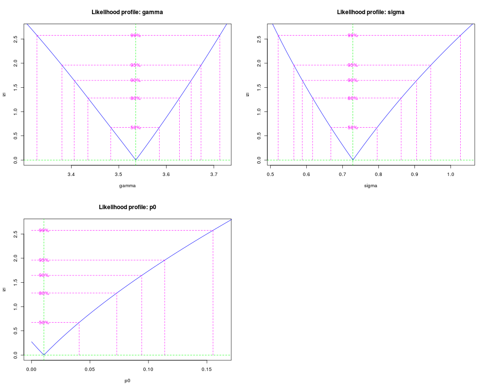
# Plot the log likelihood profiles retroactively, because before
# we set plot = FALSE
plot_RLum(mam)

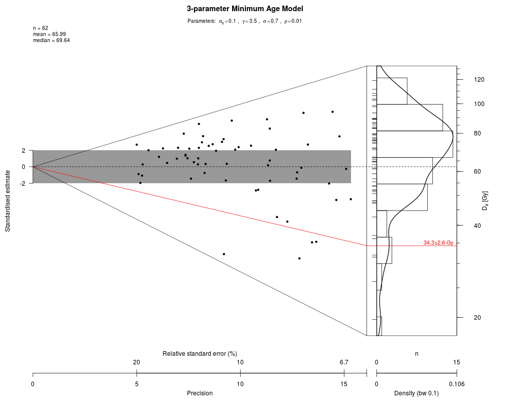
# Plot the dose distribution in an abanico plot and draw a line
# at the minimum dose estimate
plot_AbanicoPlot(data = ExampleData.DeValues$CA1,
                 main = "3-parameter Minimum Age Model",
                 line = mam,polygon.col = "none",
                 hist = TRUE,
                 rug = TRUE,
                 summary = c("n", "mean", "mean.weighted", "median", "in.ci"),
                 centrality = res$de,
                 line.col = "red",
                 grid.col = "none",
                 line.label = paste0(round(res$de, 1), "U00B1",
                                     round(res$de_err, 1), " Gy"),
                 bw = 0.1,
                 ylim = c(-25, 18),
                 summary.pos = "topleft",
                 mtext = bquote("Parameters: " ~
                                  sigma[b] == .(get_RLum(mam, "args")$sigmab) ~ ", " ~
                                  gamma == .(round(log(res$de), 1)) ~ ", " ~
                                  sigma == .(round(res$sig, 1)) ~ ", " ~
                                  rho == .(round(res$p0, 2))))


## Not run: 
# (3) Run the minimum age model with bootstrap
# NOTE: Bootstrapping is computationally intensive
# (3.1) run the minimum age model with default values for bootstrapping
calc_MinDose(data = ExampleData.DeValues$CA1,
             sigmab = 0.15,
             bootstrap = TRUE)

# (3.2) Bootstrap control parameters
mam <- calc_MinDose(data = ExampleData.DeValues$CA1,
                    sigmab = 0.15,
                    bootstrap = TRUE,
                    bs.M = 300,
                    bs.N = 500,
                    bs.h = 4,
                    sigmab.sd = 0.06,
                    plot = FALSE)

# Plot the results
plot_RLum(mam)

# save bootstrap results in a separate variable
bs <- get_RLum(mam, "bootstrap")

# show structure of the bootstrap results
str(bs, max.level = 2, give.attr = FALSE)

# print summary of minimum dose and likelihood pairs
summary(bs$pairs$gamma)

# Show polynomial fits of the bootstrap pairs
bs$poly.fits$poly.three

# Plot various statistics of the fit using the generic plot() function
par(mfcol=c(2,2))
plot(bs$poly.fits$poly.three, ask = FALSE)

# Show the fitted values of the polynomials
summary(bs$poly.fits$poly.three$fitted.values)

## End(Not run)

Results

R version 3.3.1 (2016-06-21) -- "Bug in Your Hair"
Copyright (C) 2016 The R Foundation for Statistical Computing
Platform: x86_64-pc-linux-gnu (64-bit)

R is free software and comes with ABSOLUTELY NO WARRANTY.
You are welcome to redistribute it under certain conditions.
Type 'license()' or 'licence()' for distribution details.

R is a collaborative project with many contributors.
Type 'contributors()' for more information and
'citation()' on how to cite R or R packages in publications.

Type 'demo()' for some demos, 'help()' for on-line help, or
'help.start()' for an HTML browser interface to help.
Type 'q()' to quit R.

> library(Luminescence)
Welcome to the R package Luminescence version 0.6.0 [Built: 2016-05-30 16:47:30 UTC]
An unbiased reviewer: 'The data is too poor to be published in QG, try a higher ranked journal.'
> png(filename="/home/ddbj/snapshot/RGM3/R_CC/result/Luminescence/calc_MinDose.Rd_%03d_medium.png", width=480, height=480)
> ### Name: calc_MinDose
> ### Title: Apply the (un-)logged minimum age model (MAM) after Galbraith et
> ###   al. (1999) to a given De distribution
> ### Aliases: calc_MinDose
> 
> ### ** Examples
> 
> 
> 
> ## Load example data
> data(ExampleData.DeValues, envir = environment())
> 
> # (1) Apply the minimum age model with minimum required parameters.
> # By default, this will apply the un-logged 3-parametric MAM.
> calc_MinDose(data = ExampleData.DeValues$CA1, sigmab = 0.1)

----------- meta data -----------
  n par sigmab logged      Lmax      BIC
 62   3    0.1   TRUE -43.57969 106.4405

--- final parameter estimates ---
 gamma sigma   p0 mu
  3.54  0.73 0.01  0

------ confidence intervals -----
      2.5 % 97.5 %
gamma  3.38   3.67
sigma  0.57   0.94
p0       NA   0.11

------ De (asymmetric error) -----
    De lower upper
 34.32 29.38 39.38

------ De (symmetric error) -----
    De error
 34.32  2.55
> 
> # (2) Re-run the model, but save results to a variable and turn
> # plotting of the log-likelihood profiles off.
> mam <- calc_MinDose(data = ExampleData.DeValues$CA1,
+                     sigmab = 0.1,
+                     plot = FALSE)

----------- meta data -----------
  n par sigmab logged      Lmax      BIC
 62   3    0.1   TRUE -43.57969 106.4405

--- final parameter estimates ---
 gamma sigma   p0 mu
  3.54  0.73 0.01  0

------ confidence intervals -----
      2.5 % 97.5 %
gamma  3.38   3.67
sigma  0.57   0.94
p0       NA   0.11

------ De (asymmetric error) -----
    De lower upper
 34.32 29.38 39.38

------ De (symmetric error) -----
    De error
 34.32  2.55
> 
> # Show structure of the RLum.Results object
> mam

 [RLum.Results]
	 originator: calc_MinDose()
	 data: 9
 	 .. $summary : data.frame
	 .. $data : data.frame
	 .. $args : list
	 .. $call : call
	 .. $mle : mle2
	 .. $BIC : numeric
	 .. $confint : data.frame
	 .. $profile : profile.mle2
	 .. $bootstrap : list
	 additional info elements:  0> 
> # Show summary table that contains the most relevant results
> res <- get_RLum(mam, "summary")
> res
        de   de_err ci_level ci_lower ci_upper par       sig         p0 mu
1 34.31834 2.550964     0.95 29.37526 39.37503   3 0.7287325 0.01053938 NA
       Lmax      BIC
1 -43.57969 106.4405
> 
> # Plot the log likelihood profiles retroactively, because before
> # we set plot = FALSE
> plot_RLum(mam)
> 
> # Plot the dose distribution in an abanico plot and draw a line
> # at the minimum dose estimate
> plot_AbanicoPlot(data = ExampleData.DeValues$CA1,
+                  main = "3-parameter Minimum Age Model",
+                  line = mam,polygon.col = "none",
+                  hist = TRUE,
+                  rug = TRUE,
+                  summary = c("n", "mean", "mean.weighted", "median", "in.ci"),
+                  centrality = res$de,
+                  line.col = "red",
+                  grid.col = "none",
+                  line.label = paste0(round(res$de, 1), "U00B1",
+                                      round(res$de_err, 1), " Gy"),
+                  bw = 0.1,
+                  ylim = c(-25, 18),
+                  summary.pos = "topleft",
+                  mtext = bquote("Parameters: " ~
+                                   sigma[b] == .(get_RLum(mam, "args")$sigmab) ~ ", " ~
+                                   gamma == .(round(log(res$de), 1)) ~ ", " ~
+                                   sigma == .(round(res$sig, 1)) ~ ", " ~
+                                   rho == .(round(res$p0, 2))))
> 
> 
> ## Not run: 
> ##D # (3) Run the minimum age model with bootstrap
> ##D # NOTE: Bootstrapping is computationally intensive
> ##D # (3.1) run the minimum age model with default values for bootstrapping
> ##D calc_MinDose(data = ExampleData.DeValues$CA1,
> ##D              sigmab = 0.15,
> ##D              bootstrap = TRUE)
> ##D 
> ##D # (3.2) Bootstrap control parameters
> ##D mam <- calc_MinDose(data = ExampleData.DeValues$CA1,
> ##D                     sigmab = 0.15,
> ##D                     bootstrap = TRUE,
> ##D                     bs.M = 300,
> ##D                     bs.N = 500,
> ##D                     bs.h = 4,
> ##D                     sigmab.sd = 0.06,
> ##D                     plot = FALSE)
> ##D 
> ##D # Plot the results
> ##D plot_RLum(mam)
> ##D 
> ##D # save bootstrap results in a separate variable
> ##D bs <- get_RLum(mam, "bootstrap")
> ##D 
> ##D # show structure of the bootstrap results
> ##D str(bs, max.level = 2, give.attr = FALSE)
> ##D 
> ##D # print summary of minimum dose and likelihood pairs
> ##D summary(bs$pairs$gamma)
> ##D 
> ##D # Show polynomial fits of the bootstrap pairs
> ##D bs$poly.fits$poly.three
> ##D 
> ##D # Plot various statistics of the fit using the generic plot() function
> ##D par(mfcol=c(2,2))
> ##D plot(bs$poly.fits$poly.three, ask = FALSE)
> ##D 
> ##D # Show the fitted values of the polynomials
> ##D summary(bs$poly.fits$poly.three$fitted.values)
> ## End(Not run)
> 
> 
> 
> 
> 
> 
> dev.off()
null device 
          1 
>