R Graphical Manual

Browse All

Last data update: 2014.03.03

R: Calculation of the source dose rate via the date of...

calc_SourceDoseRate

R Documentation

Calculation of the source dose rate via the date of measurement

Description

Calculating the dose rate of the irradiation source via the date of measurement based on: source calibration date, source dose rate, dose rate error. The function returns a data.frame that provides the input argument dose_rate for the function Second2Gray.

Usage

calc_SourceDoseRate(measurement.date, calib.date, calib.dose.rate, calib.error,
  source.type = "Sr-90", dose.rate.unit = "Gy/s", predict = NULL)

Arguments

`measurement.date`	`character` or `Date` (required): date of measurement in "YYYY-MM-DD". Exceptionally, if no value is provided, the date will be set to today. The argument can be provided as vector.
`calib.date`	`character` or `Date` (required): date of source calibration in "YYYY-MM-DD"
`calib.dose.rate`	`numeric` (required): dose rate at date of calibration in Gy/s or Gy/min
`calib.error`	`numeric` (required): error of dose rate at date of calibration Gy/s or Gy/min
`source.type`	`character` (with default): specify irrdiation source (`Sr-90` or `Co-60` or `Am-214`), see details for further information
`dose.rate.unit`	`character` (with default): specify dose rate unit for input (`Gy/min` or `Gy/s`), the output is given in Gy/s as valid for the function `Second2Gray`
`predict`	`integer` (with default): option allowing to predicit the dose rate of the source over time in days set by the provided value. Starting date is the value set with `measurement.date`, e.g., `calc_SourceDoseRate(...,predict = 100)` calculates the source dose rate for the next 100 days.

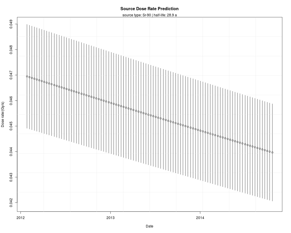
Details

Calculation of the source dose rate based on the time elapsed since the last calibration of the irradiation source. Decay parameters assume a Sr-90 beta source.

dose.rate = D0 * exp(-log(2) / T.1/2 * t)

with: D0 <- calibration dose rate T.1/2 <- half-life of the source nuclide (here in days) t <- time since source calibration (in days) log(2) / T.1/2 equals the decay constant lambda

Information on the date of measurements may be taken from the data's original .BIN file (using e.g., BINfile <- readBIN2R() and the slot BINfile@METADATA$DATE)

Allowed source types and related values

#	Source type	T.1/2	Reference
[1]	Sr-90	28.90 y	NNDC, Brookhaven National Laboratory
[2]	Am-214	432.6 y	NNDC, Brookhaven National Laboratory
[3]	Co-60	5.274 y	NNDC, Brookhaven National Laboratory

Value

Returns an S4 object of type RLum.Results. Slot data contains a list with the following structure:
$ dose.rate (data.frame)
.. $ dose.rate
.. $ dose.rate.error
.. $ date (corresponding measurement date)
$ parameters (list)
.. $ source.type
.. $ halflife
.. $ dose.rate.unit
$ call (the original function call)

The output should be accessed using the function get_RLum.
A plot method of the output is provided via plot_RLum

Function version

0.3.0 (2015-11-29 17:27:48)

Note

Please be careful when using the option predict, especially when a multiple set for measurement.date and calib.date is provided. For the source dose rate prediction the function takes the last value measurement.date and predicts from that the the source source dose rate for the number of days requested, means: the (multiple) orignal input will be replaced. However, the function do not change entries for the calibration dates, but mix them up. Therefore, it is not recommended to use this option when multiple calibration dates (calib.date) are provided.

Author(s)

Margret C. Fuchs, HZDR, Helmholtz-Institute Freiberg for Resource Technology (Germany),
Sebastian Kreutzer, IRAMAT-CRP2A, Universite Bordeaux Montaigne (France)
R Luminescence Package Team

References

NNDC, Brookhaven National Laboratory (http://www.nndc.bnl.gov/)

Examples



##(1) Simple function usage
##Basic calculation of the dose rate for a specific date
dose.rate <-  calc_SourceDoseRate(measurement.date = "2012-01-27",
                                  calib.date = "2014-12-19",
                                  calib.dose.rate = 0.0438,
                                  calib.error = 0.0019)

##show results
get_RLum(dose.rate)

##(2) Usage in combination with another function (e.g., Second2Gray() )
## load example data
data(ExampleData.DeValues, envir = environment())

## use the calculated variable dose.rate as input argument
## to convert De(s) to De(Gy)
Second2Gray(ExampleData.DeValues$BT998, dose.rate)

##(3) source rate prediction and plotting
dose.rate <-  calc_SourceDoseRate(measurement.date = "2012-01-27",
                                  calib.date = "2014-12-19",
                                  calib.dose.rate = 0.0438,
                                  calib.error = 0.0019,
                                  predict = 1000)
plot_RLum(dose.rate)


##(4) export output to a LaTeX table (example using the package 'xtable')
## Not run: 
xtable::xtable(get_RLum(dose.rate))


## End(Not run)

Results


R version 3.3.1 (2016-06-21) -- "Bug in Your Hair"
Copyright (C) 2016 The R Foundation for Statistical Computing
Platform: x86_64-pc-linux-gnu (64-bit)

R is free software and comes with ABSOLUTELY NO WARRANTY.
You are welcome to redistribute it under certain conditions.
Type 'license()' or 'licence()' for distribution details.

R is a collaborative project with many contributors.
Type 'contributors()' for more information and
'citation()' on how to cite R or R packages in publications.

Type 'demo()' for some demos, 'help()' for on-line help, or
'help.start()' for an HTML browser interface to help.
Type 'q()' to quit R.

> library(Luminescence)
Welcome to the R package Luminescence version 0.6.0 [Built: 2016-05-30 16:47:30 UTC]
A blue LED to a trapped electron: 'Resistance is futile.'
> png(filename="/home/ddbj/snapshot/RGM3/R_CC/result/Luminescence/calc_SourceDoseRate.Rd_%03d_medium.png", width=480, height=480)
> ### Name: calc_SourceDoseRate
> ### Title: Calculation of the source dose rate via the date of measurement
> ### Aliases: calc_SourceDoseRate
> ### Keywords: manip
> 
> ### ** Examples
> 
> 
> 
> ##(1) Simple function usage
> ##Basic calculation of the dose rate for a specific date
> dose.rate <-  calc_SourceDoseRate(measurement.date = "2012-01-27",
+                                   calib.date = "2014-12-19",
+                                   calib.dose.rate = 0.0438,
+                                   calib.error = 0.0019)
> 
> ##show results
> get_RLum(dose.rate)
   dose.rate dose.rate.error       date
1 0.04695031     0.002036657 2012-01-27
> 
> ##(2) Usage in combination with another function (e.g., Second2Gray() )
> ## load example data
> data(ExampleData.DeValues, envir = environment())
> 
> ## use the calculated variable dose.rate as input argument
> ## to convert De(s) to De(Gy)
> Second2Gray(ExampleData.DeValues$BT998, dose.rate)
       De De.error
1  162.37    5.717
2  163.02    5.514
3  177.72    7.294
4  145.94    4.939
5  154.81    4.976
6  132.32    4.792
7  132.54    4.531
8  136.21    4.712
9  134.05    4.963
10 133.40    4.562
11 127.13    4.340
12 137.29    4.725
13 118.75    3.967
14 129.72    4.488
15 133.01    4.426
16 133.67    4.334
17 132.57    4.568
18 135.43    4.532
19 137.84    4.560
20 140.91    4.768
21 136.96    4.641
22 140.47    5.384
23 135.43    4.628
24 123.79    3.729
25 128.18    4.090
> 
> ##(3) source rate prediction and plotting
> dose.rate <-  calc_SourceDoseRate(measurement.date = "2012-01-27",
+                                   calib.date = "2014-12-19",
+                                   calib.dose.rate = 0.0438,
+                                   calib.error = 0.0019,
+                                   predict = 1000)
> plot_RLum(dose.rate)
> 
> 
> ##(4) export output to a LaTeX table (example using the package 'xtable')
> ## Not run: 
> ##D xtable::xtable(get_RLum(dose.rate))
> ##D 
> ## End(Not run)
> 
> 
> 
> 
> 
> 
> 
> dev.off()
null device 
          1 
>