Function to calculate statistic measures

Description

This function calculates a number of descriptive statistics for De-data, most fundamentally using error-weighted approaches.

Usage

calc_Statistics(data, weight.calc = "square", digits = NULL, n.MCM = 1000,
  na.rm = TRUE)

Arguments

Details

The option to use Monte Carlo Methods (n.MCM > 0) allows calculating all descriptive statistics based on random values. The distribution of these random values is based on the Normal distribution with De values as means and De_error values as one standard deviation. Increasing the number of MCM-samples linearly increases computation time. On a Lenovo X230 machine evaluation of 25 Aliquots with n.MCM = 1000 takes 0.01 s, with n = 100000, ca. 1.65 s. It might be useful to work with logarithms of these values. See Dietze et al. (2016, Quaternary Geochronology) and the function plot_AbanicoPlot for details.

Value

Returns a list with weighted and unweighted statistic measures.

Function version

0.1.6 (2016-05-16 22:14:31)

Author(s)

Michael Dietze, GFZ Potsdam (Germany)
R Luminescence Package Team

Examples

## load example data
data(ExampleData.DeValues, envir = environment())

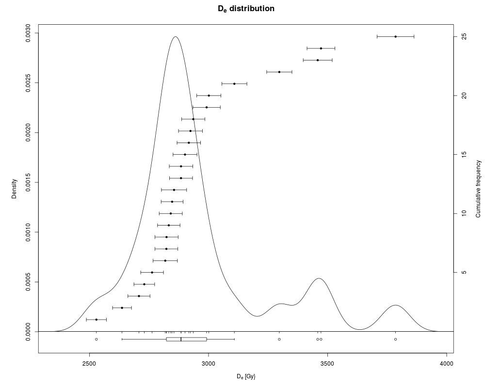
## show a rough plot of the data to illustrate the non-normal distribution
plot_KDE(ExampleData.DeValues$BT998)

## calculate statistics and show output
str(calc_Statistics(ExampleData.DeValues$BT998))

## Not run: 
## now the same for 10000 normal distributed random numbers with equal errors
x <- as.data.frame(cbind(rnorm(n = 10^5, mean = 0, sd = 1),
                         rep(0.001, 10^5)))

## note the congruent results for weighted and unweighted measures
str(calc_Statistics(x))

## End(Not run)

Results

R version 3.3.1 (2016-06-21) -- "Bug in Your Hair"
Copyright (C) 2016 The R Foundation for Statistical Computing
Platform: x86_64-pc-linux-gnu (64-bit)

R is free software and comes with ABSOLUTELY NO WARRANTY.
You are welcome to redistribute it under certain conditions.
Type 'license()' or 'licence()' for distribution details.

R is a collaborative project with many contributors.
Type 'contributors()' for more information and
'citation()' on how to cite R or R packages in publications.

Type 'demo()' for some demos, 'help()' for on-line help, or
'help.start()' for an HTML browser interface to help.
Type 'q()' to quit R.

> library(Luminescence)
Welcome to the R package Luminescence version 0.6.0 [Built: 2016-05-30 16:47:30 UTC]
A Windows user: 'An apple a day keeps the doctor away.'
> png(filename="/home/ddbj/snapshot/RGM3/R_CC/result/Luminescence/calc_Statistics.Rd_%03d_medium.png", width=480, height=480)
> ### Name: calc_Statistics
> ### Title: Function to calculate statistic measures
> ### Aliases: calc_Statistics
> ### Keywords: datagen
> 
> ### ** Examples
> 
> 
> ## load example data
> data(ExampleData.DeValues, envir = environment())
> 
> ## show a rough plot of the data to illustrate the non-normal distribution
> plot_KDE(ExampleData.DeValues$BT998)
> 
> ## calculate statistics and show output
> str(calc_Statistics(ExampleData.DeValues$BT998))
List of 3
 $ weighted  :List of 9
  ..$ n       : int 25
  ..$ mean    : num 2896
  ..$ median  : num 2884
  ..$ sd.abs  : num 240
  ..$ sd.rel  : num 8.29
  ..$ se.abs  : num 48
  ..$ se.rel  : num 1.66
  ..$ skewness: num 1.34
  ..$ kurtosis: num 4.39
 $ unweighted:List of 9
  ..$ n       : int 25
  ..$ mean    : num 2951
  ..$ median  : num 2884
  ..$ sd.abs  : num 282
  ..$ sd.rel  : num 9.54
  ..$ se.abs  : num 56.3
  ..$ se.rel  : num 1.91
  ..$ skewness: num 1.34
  ..$ kurtosis: num 4.39
 $ MCM       :List of 9
  ..$ n       : int 25
  ..$ mean    : num 2950
  ..$ median  : num 2887
  ..$ sd.abs  : num 294
  ..$ sd.rel  : num 9.98
  ..$ se.abs  : num 58.9
  ..$ se.rel  : num 2
  ..$ skewness: num 1289
  ..$ kurtosis: num 4774
> 
> ## Not run: 
> ##D ## now the same for 10000 normal distributed random numbers with equal errors
> ##D x <- as.data.frame(cbind(rnorm(n = 10^5, mean = 0, sd = 1),
> ##D                          rep(0.001, 10^5)))
> ##D 
> ##D ## note the congruent results for weighted and unweighted measures
> ##D str(calc_Statistics(x))
> ## End(Not run)
> 
> 
> 
> 
> 
> 
> dev.off()
null device 
          1 
>