Calculates the Thermal Lifetime using the Arrhenius equation

Description

The function calculates the thermal lifetime of charges for given E (in eV), s (in 1/s) and T (in deg. C.) parameters. The function can be used in two operational modes:

Usage

calc_ThermalLifetime(E, s, T = 20, output_unit = "Ma", profiling = FALSE,
  profiling_config = NULL, verbose = TRUE, plot = TRUE, ...)

Arguments

Details

Mode 1 (profiling = FALSE)

An arbitrary set of input parameters (E, s, T) can be provided and the function calculates the thermal lifetimes using the Arrhenius equation for all possible combinations of these input parameters. An array with 3-dimensions is returned that can be used for further analyses or graphical output (see example 1)

Mode 2 (profiling = TRUE)

This mode tries to profile the variation of the thermal lifetime for a chosen temperature by accounting for the provided E and s parameters and their corresponding standard errors, e.g., E = c(1.600, 0.001) The calculation based on a Monte Carlo simulation, where values are sampled from a normal distribution (for E and s).

Used equation (Arrhenius equation)

τ = 1/s exp(E/kT)

where: τ in s as the mean time an electron spends in the trap for a given T, E trap depth in eV, s the frequency factor in 1/s, T the temperature in K and k the Boltzmann constant in eV/K (cf. Furetta, 2010).

Value

A RLum.Results object is returned a along with a plot (for profiling = TRUE). The output object contain the following slots:

@data

@info

Function version

0.1.0 (2016-05-02 09:36:06)

Note

The profiling is currently based on resampling from a normal distribution, this distribution assumption might be, however, not valid for given E and s paramters.

Author(s)

Sebastian Kreutzer, IRAMAT-CRP2A, Universite Bordeaux Montaigne (France)
R Luminescence Package Team

References

Furetta, C., 2010. Handbook of Thermoluminescence, Second Edition. ed. World Scientific.

See Also

matplot, rnorm, get_RLum,

Examples

##EXAMPLE 1
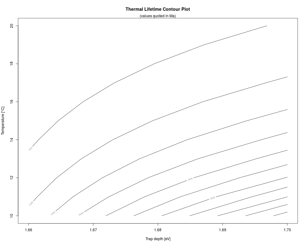
##calculation for two trap-depths with similar frequency factor for different temperatures
E <- c(1.66, 1.70)
s <- 1e+13
T <- 10:20
temp <- calc_ThermalLifetime(
  E = E,
  s = s,
  T = T,
  output_unit = "Ma"
)
contour(x = E, y = T, z = temp$lifetimes[1,,],
        ylab = "Temperature [u00B0C]",
        xlab = "Trap depth [eV]",
        main = "Thermal Lifetime Contour Plot"
)
mtext(side = 3, "(values quoted in Ma)")

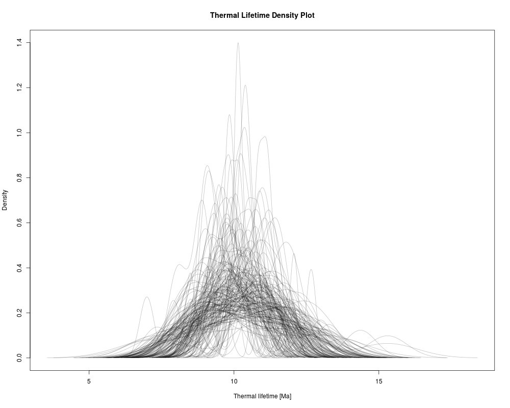
##EXAMPLE 2
##profiling of thermal life time for E and s and their standard error
E <- c(1.600, 0.003)
s <- c(1e+13,1e+011)
T <- 20
calc_ThermalLifetime(
  E = E,
  s = s,
  T = T,
  profiling = TRUE,
  output_unit = "Ma"
)

Results

R version 3.3.1 (2016-06-21) -- "Bug in Your Hair"
Copyright (C) 2016 The R Foundation for Statistical Computing
Platform: x86_64-pc-linux-gnu (64-bit)

R is free software and comes with ABSOLUTELY NO WARRANTY.
You are welcome to redistribute it under certain conditions.
Type 'license()' or 'licence()' for distribution details.

R is a collaborative project with many contributors.
Type 'contributors()' for more information and
'citation()' on how to cite R or R packages in publications.

Type 'demo()' for some demos, 'help()' for on-line help, or
'help.start()' for an HTML browser interface to help.
Type 'q()' to quit R.

> library(Luminescence)
Welcome to the R package Luminescence version 0.6.0 [Built: 2016-05-30 16:47:30 UTC]
A PhD supervisor: 'You are not depressive, you simply have a crappy life.'
> png(filename="/home/ddbj/snapshot/RGM3/R_CC/result/Luminescence/calc_ThermalLifetime.Rd_%03d_medium.png", width=480, height=480)
> ### Name: calc_ThermalLifetime
> ### Title: Calculates the Thermal Lifetime using the Arrhenius equation
> ### Aliases: calc_ThermalLifetime
> ### Keywords: datagen
> 
> ### ** Examples
> 
> 
> ##EXAMPLE 1
> ##calculation for two trap-depths with similar frequency factor for different temperatures
> E <- c(1.66, 1.70)
> s <- 1e+13
> T <- 10:20
> temp <- calc_ThermalLifetime(
+   E = E,
+   s = s,
+   T = T,
+   output_unit = "Ma"
+ )

[calc_ThermalLifetime()]

	mean:	 1.355559e+03 Ma
	sd:	 1.51684e+03 Ma
	min:	 1.095458e+02 Ma (@20 <U+00B0>C)
	max:	 5.747042e+03 Ma (@10 <U+00B0>C)
	--------------------------
	(22 lifetimes calculated in total)> contour(x = E, y = T, z = temp$lifetimes[1,,],
+         ylab = "Temperature [u00B0C]",
+         xlab = "Trap depth [eV]",
+         main = "Thermal Lifetime Contour Plot"
+ )
> mtext(side = 3, "(values quoted in Ma)")
> 
> ##EXAMPLE 2
> ##profiling of thermal life time for E and s and their standard error
> E <- c(1.600, 0.003)
> s <- c(1e+13,1e+011)
> T <- 20
> calc_ThermalLifetime(
+   E = E,
+   s = s,
+   T = T,
+   profiling = TRUE,
+   output_unit = "Ma"
+ )

[calc_ThermalLifetime()]

	profiling = TRUE
	--------------------------
	mean:	 1.01961e+01 Ma
	sd:	 1.219769e+00 Ma
	min:	 6.908607e+00 Ma
	max:	 1.474997e+01 Ma
	--------------------------
	(1000 lifetimes calculated in total)
 [RLum.Results]
	 originator: calc_ThermalLifetime()
	 data: 2
 	 .. $lifetimes : numeric
	 .. $profiling_matrix : matrix
	 additional info elements:  1> 
> 
> 
> 
> 
> 
> dev.off()
null device 
          1 
>