R: Nonlinear Least Squares Fit for CW-OSL curves [beta version]
fit_CWCurve
R Documentation
Nonlinear Least Squares Fit for CW-OSL curves [beta version]
Description
The function determines the weighted least-squares estimates of the
component parameters of a CW-OSL signal for a given maximum number of
components and returns various component parameters. The fitting procedure
uses the nls function with the port algorithm.
RLum.Data.Curve or data.frame
(required): x, y data of measured values (time and counts). See
examples.
n.components.max
vector (optional): maximum number of
components that are to be used for fitting. The upper limit is 7.
fit.failure_threshold
vector (with default): limits the failed
fitting attempts.
fit.method
character (with default): select fit method,
allowed values: 'port' and 'LM'. 'port' uses the 'port'
routine usint the funtion nls'LM' utilises the
function nlsLM from the package minpack.lm and with that the
Levenberg-Marquardt algorithm.
fit.trace
logical (with default): traces the fitting process
on the terminal.
fit.calcError
logical (with default): calculate 1-sigma error
range of components using confint
LED.power
numeric (with default): LED power (max.) used for
intensity ramping in mW/cm^2. Note: The value is used for the
calculation of the absolute photoionisation cross section.
LED.wavelength
numeric (with default): LED wavelength used for
stimulation in nm. Note: The value is used for the calculation of the
absolute photoionisation cross section.
cex.global
numeric (with default): global scaling factor.
sample_code
character (optional): sample code used for the
plot and the optional output table (mtext).
output.path
character (optional): output path for table output
containing the results of the fit. The file name is set automatically. If
the file already exists in the directory, the values are appended.
output.terminal
logical (with default): terminal ouput with
fitting results.
output.terminalAdvanced
logical (with default): enhanced
terminal output. Requires output.terminal = TRUE. If
output.terminal = FALSE no advanced output is possible.
plot
logical (with default): returns a plot of the fitted
curves.
...
further arguments and graphical parameters passed to
plot.
Details
Fitting function
The function for the CW-OSL fitting has the
general form:
y = I0_{1}*λ_{1}*exp(-λ_1*x) + ,…, +
I0_{i}*λ_{i}*exp(-λ_i*x)
where 0 < i < 8
and
λ is the decay constant and N0 the intial number of
trapped electrons. (for the used equation cf. Boetter-Jensen et al.,
2003)
Start values
Start values are estimated automatically by fitting a linear function to the
logarithmized input data set. Currently, there is no option to manually
provide start parameters.
Goodness of fit
The goodness
of the fit is given as pseudoR^2 value (pseudo coefficient of
determination). According to Lave (1970), the value is calculated as:
pseudoR^2 = 1 - RSS/TSS
where RSS = Residual~Sum~of~Squares
and TSS = Total~Sum~of~Squares
Error of fitted component parameters
The 1-sigma error for the
components is calculated using the function confint. Due to
considerable calculation time, this option is deactived by default. In
addition, the error for the components can be estimated by using internal R
functions like summary. See the nls help page
for more information.
For details on the nonlinear regression in
R, see Ritz & Streibig (2008).
Value
plot
(optional) the fitted CW-OSL curves are returned as
plot.
table
(optional) an output table (*.csv) with parameters of
the fitted components is provided if the output.path is set.
list(list("RLum.Results"))
beside the plot and table output options,
an RLum.Results object is returned.
fit:
an nls object ($fit) for which generic R functions are
provided, e.g. summary, confint, profile. For more
details, see nls.
output.table: a data.frame
containing the summarised parameters including the error component.contribution.matrix: matrix containing the values
for the component to sum contribution plot
($component.contribution.matrix).
Matrix structure: Column 1 and 2: time and rev(time) values
Additional columns are used for the components, two for each component,
containing I0 and n0. The last columns cont. provide information on
the relative component contribution for each time interval including the row
sum for this values.
object
beside the plot and table output
options, an RLum.Results object is returned.
fit: an nls object ($fit) for which generic R functions
are provided, e.g. summary, confint, profile. For more
details, see nls.
output.table: a data.frame
containing the summarised parameters including the error component.contribution.matrix: matrix containing the values
for the component to sum contribution plot
($component.contribution.matrix).
Matrix structure: Column 1 and 2: time and rev(time) values
Additional columns are used for the components, two for each component,
containing I0 and n0. The last columns cont. provide information on
the relative component contribution for each time interval including the row
sum for this values.
Function version
0.5.1 (2015-11-29 17:27:48)
Note
Beta version - This function has not been properly tested yet
and should therefore not be used for publication purposes!
The
pseudo-R^2 may not be the best parameter to describe the goodness of the
fit. The trade off between the n.components and the pseudo-R^2 value
is currently not considered.
The function does not ensure that
the fitting procedure has reached a global minimum rather than a local
minimum!
Author(s)
Sebastian Kreutzer, IRAMAT-CRP2A, Universite Bordeaux Montaigne
(France)
R Luminescence Package Team
##load data
data(ExampleData.CW_OSL_Curve, envir = environment())
##fit data
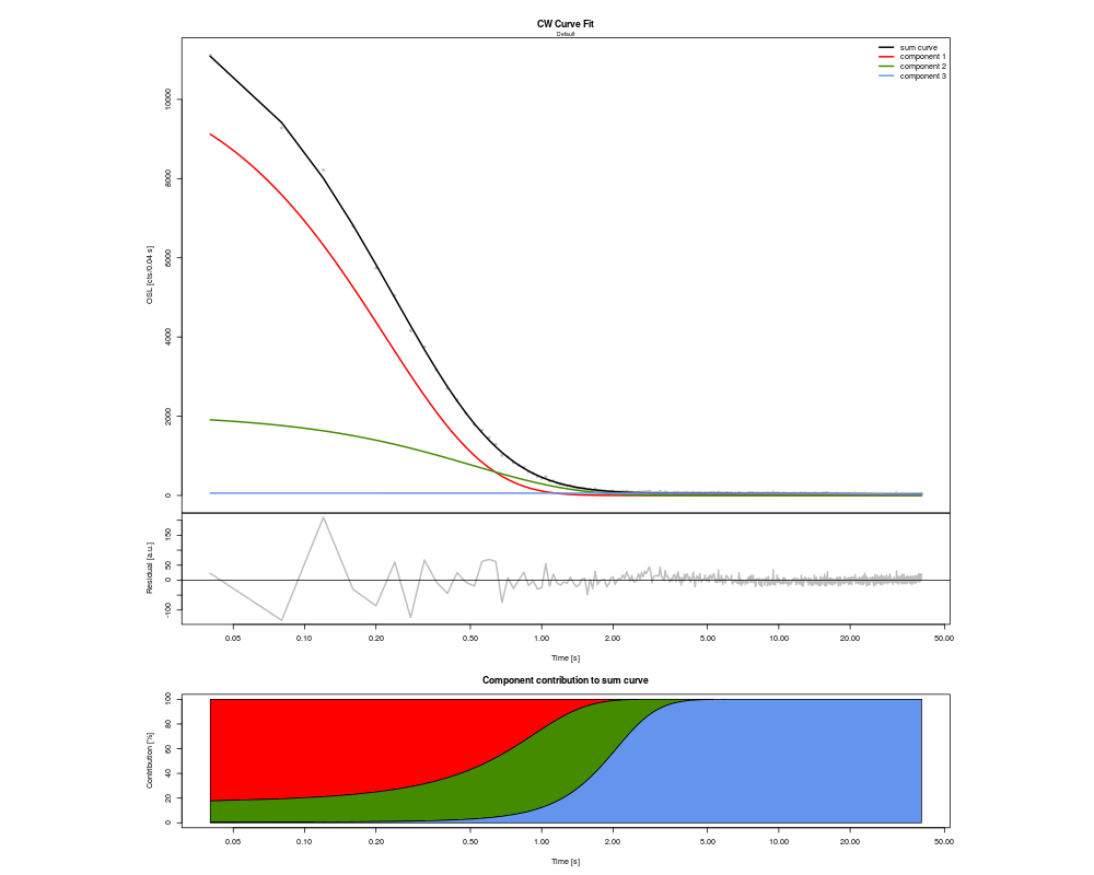
fit <- fit_CWCurve(values = ExampleData.CW_OSL_Curve,
main = "CW Curve Fit",
n.components.max = 4,
log = "x")
Results
R version 3.3.1 (2016-06-21) -- "Bug in Your Hair"
Copyright (C) 2016 The R Foundation for Statistical Computing
Platform: x86_64-pc-linux-gnu (64-bit)

R is free software and comes with ABSOLUTELY NO WARRANTY.
You are welcome to redistribute it under certain conditions.
Type 'license()' or 'licence()' for distribution details.

R is a collaborative project with many contributors.
Type 'contributors()' for more information and
'citation()' on how to cite R or R packages in publications.

Type 'demo()' for some demos, 'help()' for on-line help, or
'help.start()' for an HTML browser interface to help.
Type 'q()' to quit R.

> library(Luminescence)
Welcome to the R package Luminescence version 0.6.0 [Built: 2016-05-30 16:47:30 UTC]
A weathering rock: 'Who wants to live forever?'
> png(filename="/home/ddbj/snapshot/RGM3/R_CC/result/Luminescence/fit_CWCurve.Rd_%03d_medium.png", width=480, height=480)
> ### Name: fit_CWCurve
> ### Title: Nonlinear Least Squares Fit for CW-OSL curves [beta version]
> ### Aliases: fit_CWCurve
> ### Keywords: dplot models
>
> ### ** Examples
>
>
>
> ##load data
> data(ExampleData.CW_OSL_Curve, envir = environment())
>
> ##fit data
> fit <- fit_CWCurve(values = ExampleData.CW_OSL_Curve,
+                    main = "CW Curve Fit",
+                    n.components.max = 4,
+                    log = "x")

[fit_CWCurve()]

Fitting was finally done using a 3-component function (max=4):
------------------------------------------------------------------------------
y ~ I0.1 * lambda.1 * exp(-lambda.1 * x) + I0.2 * lambda.2 * exp(-lambda.2 * x) + I0.3 * lambda.3 * exp(-lambda.3 * x)

         I0 I0.error     lambda lambda.error           cs cs.rel
c1 2387.617       NA 4.59054005           NA 5.389396e-17 1.0000
c2 1053.492       NA 1.95936493           NA 2.300338e-17 0.4268
c3 2816.629       NA 0.02054734           NA 2.412303e-19 0.0045
------------------------------------------------------------------------------
pseudo-R^2 = 0.9995
>
>
>
>
>
>
> dev.off()
null device
          1
>
 .
.