Nonlinear Least Squares Fit for LM-OSL curves

Description

The function determines weighted nonlinear least-squares estimates of the component parameters of an LM-OSL curve (Bulur 1996) for a given number of components and returns various component parameters. The fitting procedure uses the function nls with the port algorithm.

Usage

fit_LMCurve(values, values.bg, n.components = 3, start_values,
  input.dataType = "LM", fit.method = "port", sample_code = "",
  sample_ID = "", LED.power = 36, LED.wavelength = 470,
  fit.trace = FALSE, fit.advanced = FALSE, fit.calcError = FALSE,
  bg.subtraction = "polynomial", verbose = TRUE, plot = TRUE,
  plot.BG = FALSE, ...)

Arguments

Details

Fitting function

The function for the fitting has the general form:

y = (exp(0.5)*Im_1*x/xm_1)*exp(-x^2/(2*xm_1^2)) + ,…, + exp(0.5)*Im_i*x/xm_i)*exp(-x^2/(2*xm_i^2))

where 1 < i < 8
This function and the equations for the conversion to b (detrapping probability) and n0 (proportional to initially trapped charge) have been taken from Kitis et al. (2008):

xm_i=√{max(t)/b_i}

Im_i=exp(-0.5)n0/xm_i

Background subtraction

Three methods for background subtraction are provided for a given background signal (values.bg).
polynomial: default method. A polynomial function is fitted using glm and the resulting function is used for background subtraction:

y = a*x^4 + b*x^3 + c*x^2 + d*x + e

linear: a linear function is fitted using glm and the resulting function is used for background subtraction:

y = a*x + b

channel: the measured background signal is subtracted channelwise from the measured signal.

Start values

The choice of the initial parameters for the nls-fitting is a crucial point and the fitting procedure may mainly fail due to ill chosen start parameters. Here, three options are provided:

(a) If no start values (start_values) are provided by the user, a cheap guess is made by using the detrapping values found by Jain et al. (2003) for quartz for a maximum of 7 components. Based on these values, the pseudo start parameters xm and Im are recalculated for the given data set. In all cases, the fitting starts with the ultra-fast component and (depending on n.components) steps through the following values. If no fit could be achieved, an error plot (for plot = TRUE) with the pseudo curve (based on the pseudo start parameters) is provided. This may give the opportunity to identify appropriate start parameters visually.

(b) If start values are provided, the function works like a simple nls fitting approach.

(c) If no start parameters are provided and the option fit.advanced = TRUE is chosen, an advanced start paramter estimation is applied using a stochastical attempt. Therefore, the recalculated start parameters (a) are used to construct a normal distribution. The start parameters are then sampled randomly from this distribution. A maximum of 100 attempts will be made. Note: This process may be time consuming.

Goodness of fit

The goodness of the fit is given by a pseudoR^2 value (pseudo coefficient of determination). According to Lave (1970), the value is calculated as:

pseudoR^2 = 1 - RSS/TSS

where RSS = Residual~Sum~of~Squares
and TSS = Total~Sum~of~Squares

Error of fitted component parameters

The 1-sigma error for the components is calculated using the function confint. Due to considerable calculation time, this option is deactived by default. In addition, the error for the components can be estimated by using internal R functions like summary. See the nls help page for more information.
For more details on the nonlinear regression in R, see Ritz & Streibig (2008).

Value

Various types of plots are returned. For details see above.
Furthermore an RLum.Results object is returned with the following structure:

data:
.. $fit : nls (nls object)
.. $output.table : data.frame with fitting results
.. $component.contribution.matrix : list component distribution matrix
.. $call : call the original function call

Matrix structure for the distribution matrix:

Column 1 and 2: time and rev(time) values
Additional columns are used for the components, two for each component, containing I0 and n0. The last columns cont. provide information on the relative component contribution for each time interval including the row sum for this values.

Function version

0.3.1 (2016-05-02 09:36:06)

Note

The pseudo-R^2 may not be the best parameter to describe the goodness of the fit. The trade off between the n.components and the pseudo-R^2 value currently remains unconsidered.

The function does not ensure that the fitting procedure has reached a global minimum rather than a local minimum! In any case of doubt, the use of manual start values is highly recommended.

Author(s)

Sebastian Kreutzer, IRAMAT-CRP2A, Universite Bordeaux Montaigne (France)
R Luminescence Package Team

References

Bulur, E., 1996. An Alternative Technique For Optically Stimulated Luminescence (OSL) Experiment. Radiation Measurements, 26, 5, 701-709.

Jain, M., Murray, A.S., Boetter-Jensen, L., 2003. Characterisation of blue-light stimulated luminescence components in different quartz samples: implications for dose measurement. Radiation Measurements, 37 (4-5), 441-449.

Kitis, G. & Pagonis, V., 2008. Computerized curve deconvolution analysis for LM-OSL. Radiation Measurements, 43, 737-741.

Lave, C.A.T., 1970. The Demand for Urban Mass Transportation. The Review of Economics and Statistics, 52 (3), 320-323.

Ritz, C. & Streibig, J.C., 2008. Nonlinear Regression with R. R. Gentleman, K. Hornik, & G. Parmigiani, eds., Springer, p. 150.

See Also

fit_CWCurve, plot, nls, nlsLM, get_RLum

Examples

##(1) fit LM data without background subtraction
data(ExampleData.FittingLM, envir = environment())
fit_LMCurve(values = values.curve, n.components = 3, log = "x")

##(2) fit LM data with background subtraction and export as JPEG
## -alter file path for your preferred system
##jpeg(file = "~/Desktop/Fit_Output%03d.jpg", quality = 100,
## height = 3000, width = 3000, res = 300)
data(ExampleData.FittingLM, envir = environment())
fit_LMCurve(values = values.curve, values.bg = values.curveBG,
            n.components = 2, log = "x", plot.BG = TRUE)
##dev.off()

##(3) fit LM data with manual start parameters
data(ExampleData.FittingLM, envir = environment())
fit_LMCurve(values = values.curve,
            values.bg = values.curveBG,
            n.components = 3,
            log = "x",
            start_values = data.frame(Im = c(170,25,400), xm = c(56,200,1500)))

Results

R version 3.3.1 (2016-06-21) -- "Bug in Your Hair"
Copyright (C) 2016 The R Foundation for Statistical Computing
Platform: x86_64-pc-linux-gnu (64-bit)

R is free software and comes with ABSOLUTELY NO WARRANTY.
You are welcome to redistribute it under certain conditions.
Type 'license()' or 'licence()' for distribution details.

R is a collaborative project with many contributors.
Type 'contributors()' for more information and
'citation()' on how to cite R or R packages in publications.

Type 'demo()' for some demos, 'help()' for on-line help, or
'help.start()' for an HTML browser interface to help.
Type 'q()' to quit R.

> library(Luminescence)
Welcome to the R package Luminescence version 0.6.0 [Built: 2016-05-30 16:47:30 UTC]
The natural dose: 'You only life once.'
> png(filename="/home/ddbj/snapshot/RGM3/R_CC/result/Luminescence/fit_LMCurve.Rd_%03d_medium.png", width=480, height=480)
> ### Name: fit_LMCurve
> ### Title: Nonlinear Least Squares Fit for LM-OSL curves
> ### Aliases: fit_LMCurve
> ### Keywords: dplot models
> 
> ### ** Examples
> 
> 
> 
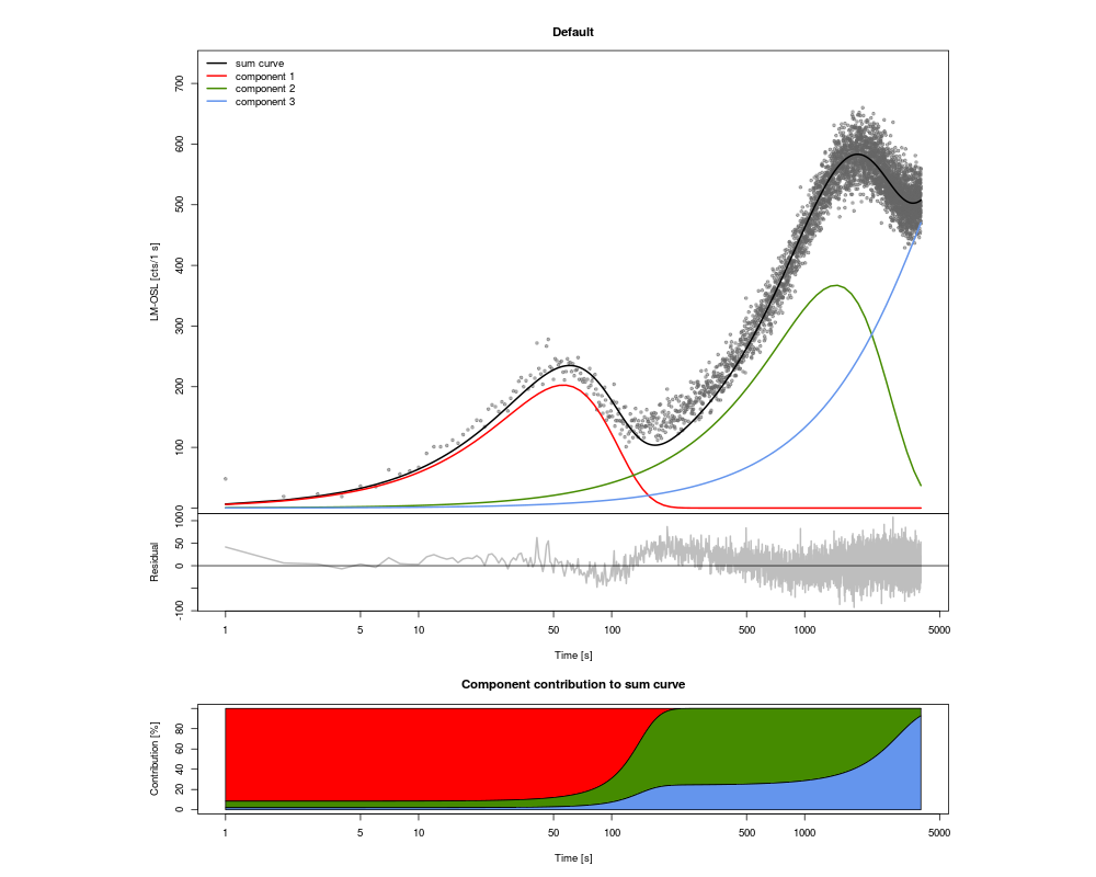
> ##(1) fit LM data without background subtraction
> data(ExampleData.FittingLM, envir = environment())
> fit_LMCurve(values = values.curve, n.components = 3, log = "x")

[fit_LMCurve()]

Fitting was done using a 3-component function:

       xm1        xm2        xm3        Im1        Im2        Im3 
  56.18289 1449.72461 7878.25139  202.76634  367.30226  639.21356 

(equation used for fitting according Kitis & Pagonis, 2008)
------------------------------------------------------------------------------
(1) Corresponding values according the equation in Bulur, 1996 for b and n0:

b1 = 1.267219e+00 +/- NA
n01 = 1.878223e+04 +/- NA

b2 = 1.90322e-03 +/- NA
n02 = 8.779229e+05 +/- NA

b3 = 6.444665e-05 +/- NA
n03 = 8.302771e+06 +/- NA

cs from component.1 = 1.488e-17 cm^2	 >> relative: 1
cs from component.2 = 2.234e-20 cm^2	 >> relative: 0.0015
cs from component.3 = 7.566e-22 cm^2	 >> relative: 1e-04

(stimulation intensity value used for calculation: 8.517726e+16 1/s 1/cm^2)
(errors quoted as 1-sigma uncertainties)
------------------------------------------------------------------------------

pseudo-R^2 = 0.9557
> 
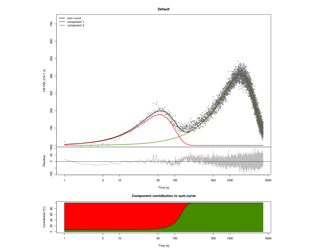
> ##(2) fit LM data with background subtraction and export as JPEG
> ## -alter file path for your preferred system
> ##jpeg(file = "~/Desktop/Fit_Output%03d.jpg", quality = 100,
> ## height = 3000, width = 3000, res = 300)
> data(ExampleData.FittingLM, envir = environment())
> fit_LMCurve(values = values.curve, values.bg = values.curveBG,
+             n.components = 2, log = "x", plot.BG = TRUE)
[fit_LMCurve] >> Background subtracted (method="polynomial")!

[fit_LMCurve()]

Fitting was done using a 2-component function:

       xm1        xm2        Im1        Im2 
  53.32071 1587.57201  176.74408  406.89925 

(equation used for fitting according Kitis & Pagonis, 2008)
------------------------------------------------------------------------------
(1) Corresponding values according the equation in Bulur, 1996 for b and n0:

b1 = 1.406916e+00 +/- NA
n01 = 1.553775e+04 +/- NA

b2 = 1.587059e-03 +/- NA
n02 = 1.065044e+06 +/- NA

cs from component.1 = 1.652e-17 cm^2	 >> relative: 1
cs from component.2 = 1.863e-20 cm^2	 >> relative: 0.0011

(stimulation intensity value used for calculation: 8.517726e+16 1/s 1/cm^2)
(errors quoted as 1-sigma uncertainties)
------------------------------------------------------------------------------

pseudo-R^2 = 0.9417
> ##dev.off()
> 
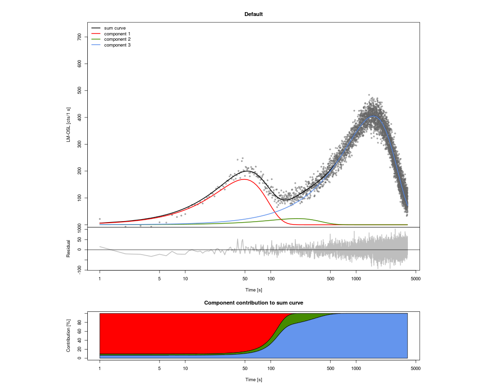
> ##(3) fit LM data with manual start parameters
> data(ExampleData.FittingLM, envir = environment())
> fit_LMCurve(values = values.curve,
+             values.bg = values.curveBG,
+             n.components = 3,
+             log = "x",
+             start_values = data.frame(Im = c(170,25,400), xm = c(56,200,1500)))
[fit_LMCurve] >> Background subtracted (method="polynomial")!

[fit_LMCurve()]

Fitting was done using a 3-component function:

       xm1        xm2        xm3        Im1        Im2        Im3 
  49.00643  204.40083 1591.66448  169.44002   23.00741  405.46171 

(equation used for fitting according Kitis & Pagonis, 2008)
------------------------------------------------------------------------------
(1) Corresponding values according the equation in Bulur, 1996 for b and n0:

b1 = 1.665536e+00 +/- NA
n01 = 1.36904e+04 +/- NA

b2 = 9.574028e-02 +/- NA
n02 = 7.753496e+03 +/- NA

b3 = 1.578908e-03 +/- NA
n03 = 1.064017e+06 +/- NA

cs from component.1 = 1.955e-17 cm^2	 >> relative: 1
cs from component.2 = 1.124e-18 cm^2	 >> relative: 0.0575
cs from component.3 = 1.854e-20 cm^2	 >> relative: 9e-04

(stimulation intensity value used for calculation: 8.517726e+16 1/s 1/cm^2)
(errors quoted as 1-sigma uncertainties)
------------------------------------------------------------------------------

pseudo-R^2 = 0.9437
> 
> 
> 
> 
> 
> 
> dev.off()
null device 
          1 
>