Supported by Dr. Osamu Ogasawara and  . . |
|
Last data update: 2014.03.03 |
Visualise dose recovery test resultsDescriptionThe function provides a standardised plot output for dose recovery test measurements. Usageplot_DRTResults(values, given.dose = NULL, error.range = 10, preheat, boxplot = FALSE, mtext, summary, summary.pos, legend, legend.pos, par.local = TRUE, na.rm = FALSE, ...) Arguments
DetailsProcedure to test the accuracy of a measurement protocol to reliably
determine the dose of a specific sample. Here, the natural signal is erased
and a known laboratory dose administered which is treated as unknown. Then
the De measurement is carried out and the degree of congruence between
administered and recovered dose is a measure of the protocol's accuracy for
this sample. ValueA plot is returned. Function version0.1.10 (2016-05-02 09:36:06) NoteFurther data and plot arguments can be added by using the appropiate R commands. Author(s)Sebastian Kreutzer, IRAMAT-CRP2A, Universite Bordeaux Montaigne
(France), Michael Dietze, GFZ Potsdam (Germany)
ReferencesWintle, A.G., Murray, A.S., 2006. A review of quartz optically stimulated luminescence characteristics and their relevance in single-aliquot regeneration dating protocols. Radiation Measurements, 41, 369-391. See Also
Examples
## read example data set and misapply them for this plot type
data(ExampleData.DeValues, envir = environment())
## plot values
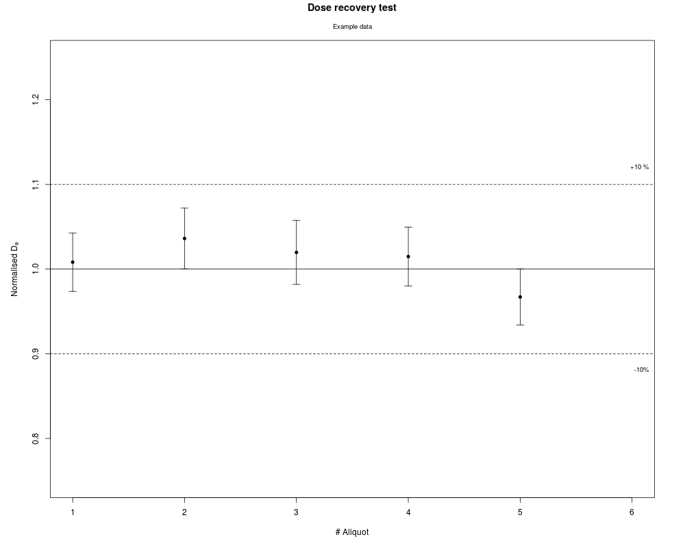
plot_DRTResults(values = ExampleData.DeValues$BT998[7:11,],
given.dose = 2800, mtext = "Example data")
## plot values with legend
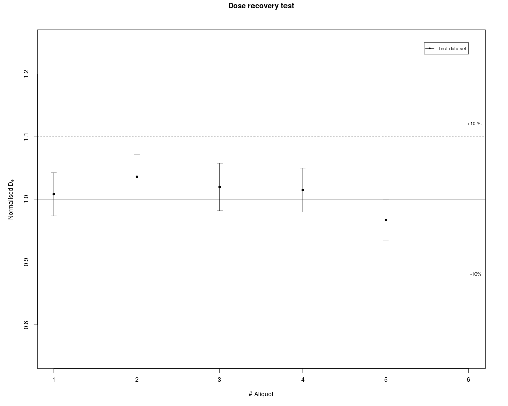
plot_DRTResults(values = ExampleData.DeValues$BT998[7:11,],
given.dose = 2800,
legend = "Test data set")
## create and plot two subsets with randomised values
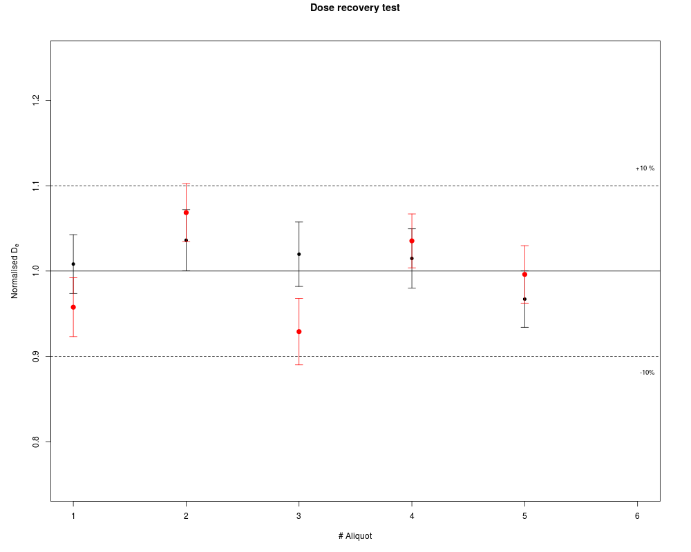
x.1 <- ExampleData.DeValues$BT998[7:11,]
x.2 <- ExampleData.DeValues$BT998[7:11,] * c(runif(5, 0.9, 1.1), 1)
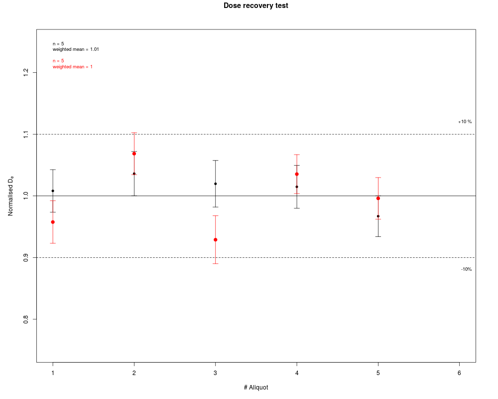
plot_DRTResults(values = list(x.1, x.2),
given.dose = 2800)
## some more user-defined plot parameters
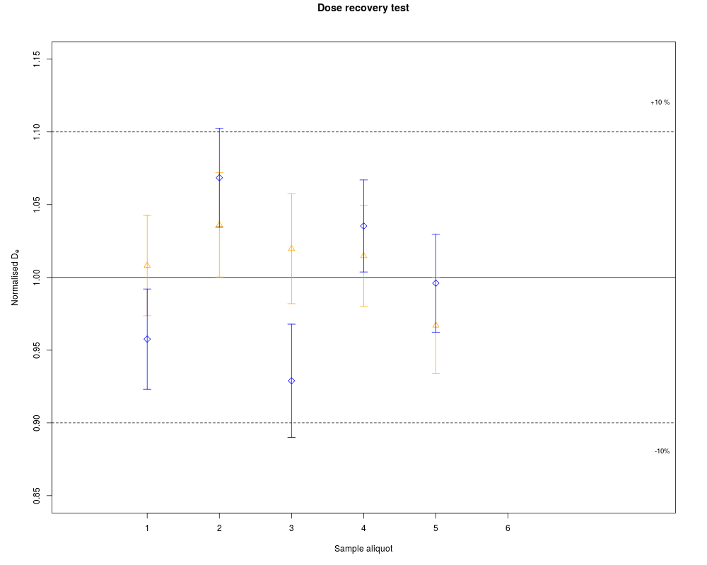
plot_DRTResults(values = list(x.1, x.2),
given.dose = 2800,
pch = c(2, 5),
col = c("orange", "blue"),
xlim = c(0, 8),
ylim = c(0.85, 1.15),
xlab = "Sample aliquot")
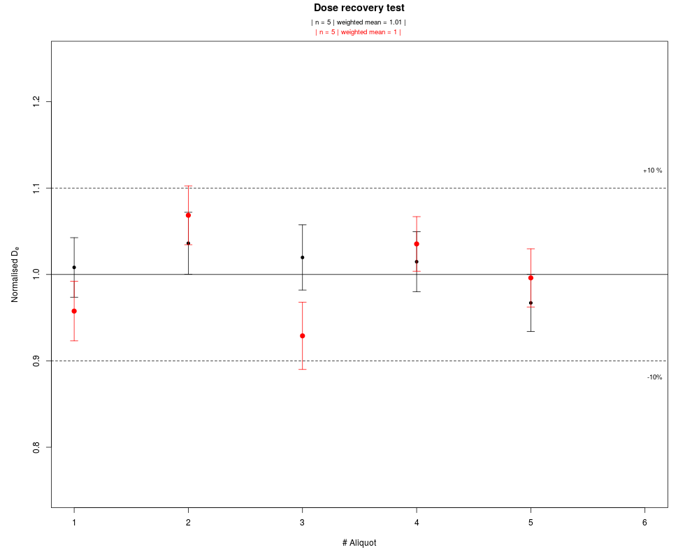
## plot the data with user-defined statistical measures as legend
plot_DRTResults(values = list(x.1, x.2),
given.dose = 2800,
summary = c("n", "mean.weighted", "sd"))
## plot the data with user-defined statistical measures as sub-header
plot_DRTResults(values = list(x.1, x.2),
given.dose = 2800,
summary = c("n", "mean.weighted", "sd"),
summary.pos = "sub")
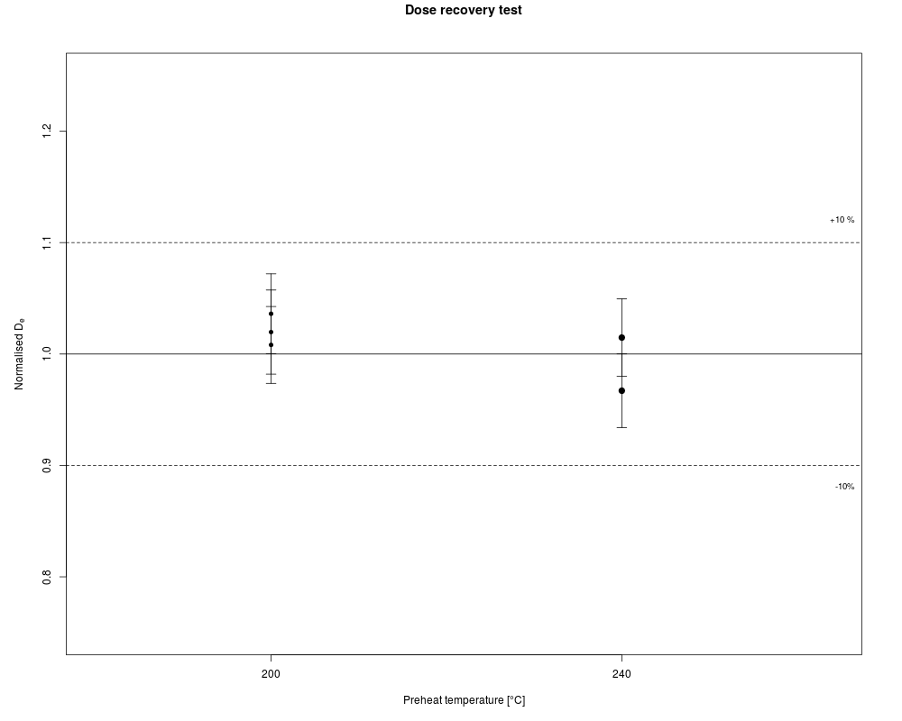
## plot the data grouped by preheat temperatures
plot_DRTResults(values = ExampleData.DeValues$BT998[7:11,],
given.dose = 2800,
preheat = c(200, 200, 200, 240, 240))
## read example data set and misapply them for this plot type
data(ExampleData.DeValues, envir = environment())
## plot values
plot_DRTResults(values = ExampleData.DeValues$BT998[7:11,],
given.dose = 2800, mtext = "Example data")
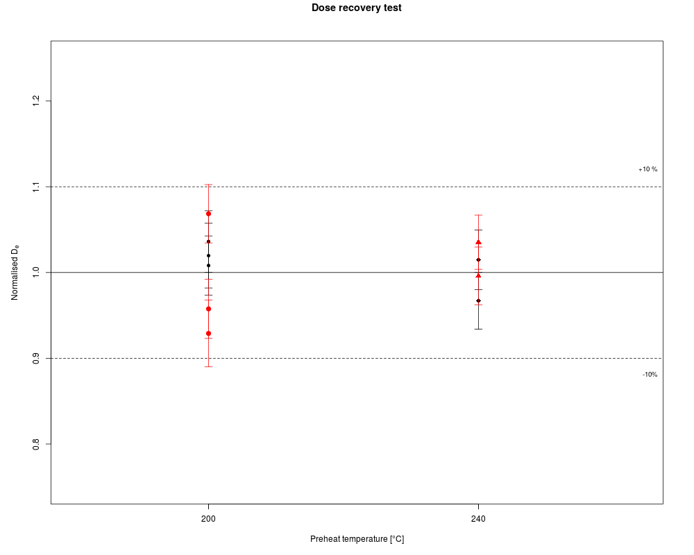
## plot two data sets grouped by preheat temperatures
plot_DRTResults(values = list(x.1, x.2),
given.dose = 2800,
preheat = c(200, 200, 200, 240, 240))
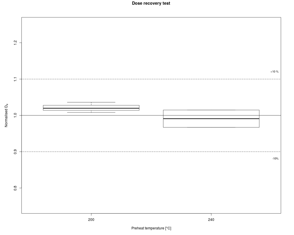
## plot the data grouped by preheat temperatures as boxplots
plot_DRTResults(values = ExampleData.DeValues$BT998[7:11,],
given.dose = 2800,
preheat = c(200, 200, 200, 240, 240),
boxplot = TRUE)
Results
R version 3.3.1 (2016-06-21) -- "Bug in Your Hair"
Copyright (C) 2016 The R Foundation for Statistical Computing
Platform: x86_64-pc-linux-gnu (64-bit)

R is free software and comes with ABSOLUTELY NO WARRANTY.
You are welcome to redistribute it under certain conditions.
Type 'license()' or 'licence()' for distribution details.

R is a collaborative project with many contributors.
Type 'contributors()' for more information and
'citation()' on how to cite R or R packages in publications.

Type 'demo()' for some demos, 'help()' for on-line help, or
'help.start()' for an HTML browser interface to help.
Type 'q()' to quit R.

> library(Luminescence)
Welcome to the R package Luminescence version 0.6.0 [Built: 2016-05-30 16:47:30 UTC]
A common luminescence reader customer: 'If anything can go wrong, it will.'
> png(filename="/home/ddbj/snapshot/RGM3/R_CC/result/Luminescence/plot_DRTResults.Rd_%03d_medium.png", width=480, height=480)
> ### Name: plot_DRTResults
> ### Title: Visualise dose recovery test results
> ### Aliases: plot_DRTResults
> ### Keywords: dplot
>
> ### ** Examples
>
>
>
> ## read example data set and misapply them for this plot type
> data(ExampleData.DeValues, envir = environment())
>
> ## plot values
> plot_DRTResults(values = ExampleData.DeValues$BT998[7:11,],
+ given.dose = 2800, mtext = "Example data")
>
> ## plot values with legend
> plot_DRTResults(values = ExampleData.DeValues$BT998[7:11,],
+                 given.dose = 2800,
+                 legend = "Test data set")
>
> ## create and plot two subsets with randomised values
> x.1 <- ExampleData.DeValues$BT998[7:11,]
> x.2 <- ExampleData.DeValues$BT998[7:11,] * c(runif(5, 0.9, 1.1), 1)
>
> plot_DRTResults(values = list(x.1, x.2),
+                 given.dose = 2800)
>
> ## some more user-defined plot parameters
> plot_DRTResults(values = list(x.1, x.2),
+                 given.dose = 2800,
+                 pch = c(2, 5),
+                 col = c("orange", "blue"),
+                 xlim = c(0, 8),
+                 ylim = c(0.85, 1.15),
+                 xlab = "Sample aliquot")
>
> ## plot the data with user-defined statistical measures as legend
> plot_DRTResults(values = list(x.1, x.2),
+                 given.dose = 2800,
+                 summary = c("n", "mean.weighted", "sd"))
>
> ## plot the data with user-defined statistical measures as sub-header
> plot_DRTResults(values = list(x.1, x.2),
+                 given.dose = 2800,
+                 summary = c("n", "mean.weighted", "sd"),
+                 summary.pos = "sub")
>
> ## plot the data grouped by preheat temperatures
> plot_DRTResults(values = ExampleData.DeValues$BT998[7:11,],
+                 given.dose = 2800,
+                 preheat = c(200, 200, 200, 240, 240))
> ## read example data set and misapply them for this plot type
> data(ExampleData.DeValues, envir = environment())
>
> ## plot values
> plot_DRTResults(values = ExampleData.DeValues$BT998[7:11,],
+                 given.dose = 2800, mtext = "Example data")
> ## plot two data sets grouped by preheat temperatures
> plot_DRTResults(values = list(x.1, x.2),
+                 given.dose = 2800,
+                 preheat = c(200, 200, 200, 240, 240))
>
> ## plot the data grouped by preheat temperatures as boxplots
> plot_DRTResults(values = ExampleData.DeValues$BT998[7:11,],
+                 given.dose = 2800,
+                 preheat = c(200, 200, 200, 240, 240),
+                 boxplot = TRUE)
>
>
>
>
>
>
> dev.off()
null device
          1
>
|