Plot filter combinations along with net transmission window

Description

The function allows to plot transmission windows for different filters. Missing data for specific wavelenghts are automatically interpolated for the given filter data using the function approx. With that a standardised output is reached and a net transmission window can be shown.

Usage

plot_FilterCombinations(filters, wavelength_range = 200:1000,
  show_net_transmission = TRUE, plot = TRUE, ...)

Arguments

Details

How to provide input data?

CASE 1

The function expects that all filter values are either of type matrix or data.frame with two columns. The first columens contains the wavelength, the second the relative transmission (but not in percentage, i.e. the maximum transmission can be only become 1).

In this case only the transmission window is show as provided. Changes in filter thickness and relection factor are not considered.

CASE 2

The filter data itself are provided as list element containing a matrix or data.frame and additional information on the thickness of the filter, e.g., list(filter1 = list(filter_matrix, d = 2)). The given filter data are always considered as standard input and the filter thickness value is taken into account by

Transmission = Transmission^(d)

with d given in the same dimension as the original filter data.

CASE 3

Same as CASE 2 but additionally a reflection factor P is provided, e.g., list(filter1 = list(filter_matrix, d = 2, P = 0.9)). The final transmission becomes:

Transmission = Transmission^(d) * P

Advanced plotting parameters

The following further non-common plotting parameters can be passed to the function:

For further modifications standard additional R plot functions are recommend, e.g., the legend can be fully customised by disabling the standard legend and use the function legend instead.

Value

Returns an S4 object of type RLum.Results.

@data

@info

Function version

0.1.0 (2016-05-02 09:36:06)

Author(s)

Sebastian Kreutzer, IRAMAT-CRP2A, Universite Bordeaux Montagine (France)

R Luminescence Package Team

See Also

RLum.Results, approx

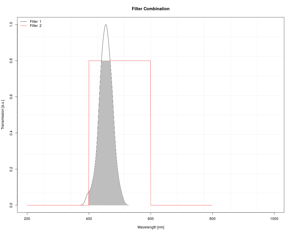
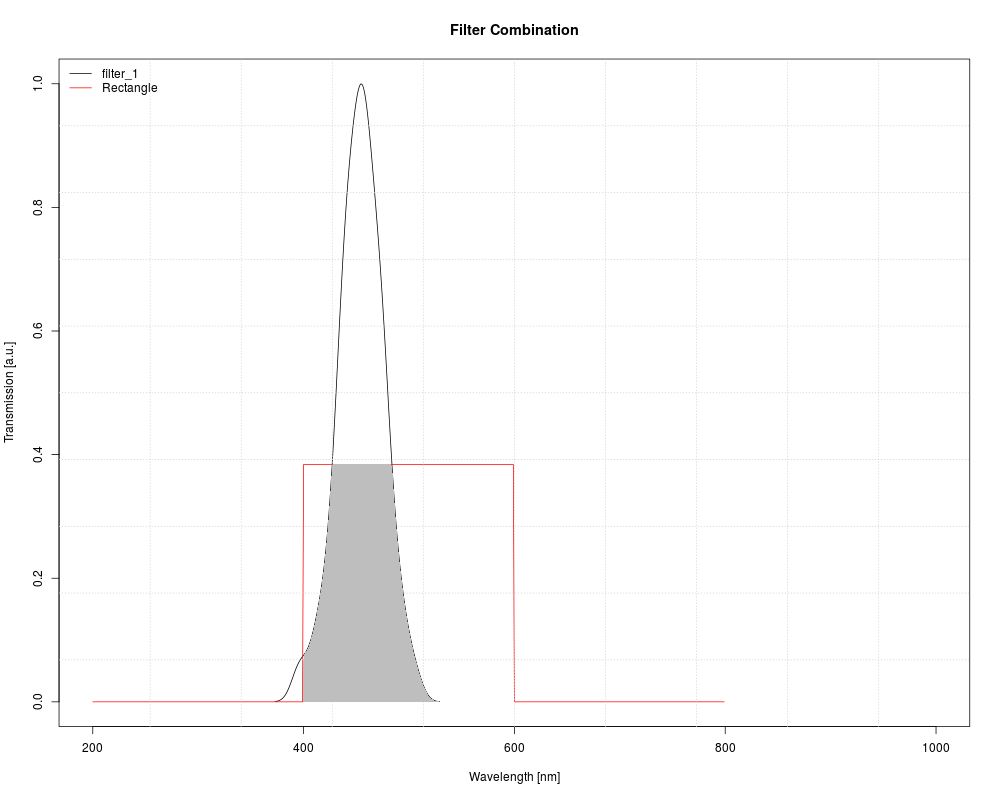
Examples

## (For legal reasons no real filter data are provided)

## Create filter sets
filter1 <- density(rnorm(100, mean = 450, sd = 20))
filter1 <- matrix(c(filter1$x, filter1$y/max(filter1$y)), ncol = 2)
filter2 <- matrix(c(200:799,rep(c(0,0.8,0),each = 200)), ncol = 2)

## Example 1 (standard)
plot_FilterCombinations(filters = list(filter1, filter2))

## Example 2 (with d and P value and name for filter 2)
results <- plot_FilterCombinations(
filters = list(filter_1 = filter1, Rectangle = list(filter2, d = 2, P = 0.6)))
results

Results

R version 3.3.1 (2016-06-21) -- "Bug in Your Hair"
Copyright (C) 2016 The R Foundation for Statistical Computing
Platform: x86_64-pc-linux-gnu (64-bit)

R is free software and comes with ABSOLUTELY NO WARRANTY.
You are welcome to redistribute it under certain conditions.
Type 'license()' or 'licence()' for distribution details.

R is a collaborative project with many contributors.
Type 'contributors()' for more information and
'citation()' on how to cite R or R packages in publications.

Type 'demo()' for some demos, 'help()' for on-line help, or
'help.start()' for an HTML browser interface to help.
Type 'q()' to quit R.

> library(Luminescence)
Welcome to the R package Luminescence version 0.6.0 [Built: 2016-05-30 16:47:30 UTC]
A Windows user: 'An apple a day keeps the doctor away.'
> png(filename="/home/ddbj/snapshot/RGM3/R_CC/result/Luminescence/plot_FilterCombinations.Rd_%03d_medium.png", width=480, height=480)
> ### Name: plot_FilterCombinations
> ### Title: Plot filter combinations along with net transmission window
> ### Aliases: plot_FilterCombinations
> ### Keywords: aplot datagen
> 
> ### ** Examples
> 
> 
> ## (For legal reasons no real filter data are provided)
> 
> ## Create filter sets
> filter1 <- density(rnorm(100, mean = 450, sd = 20))
> filter1 <- matrix(c(filter1$x, filter1$y/max(filter1$y)), ncol = 2)
> filter2 <- matrix(c(200:799,rep(c(0,0.8,0),each = 200)), ncol = 2)
> 
> ## Example 1 (standard)
> plot_FilterCombinations(filters = list(filter1, filter2))

 [RLum.Results]
	 originator: plot_FilterCombinations()
	 data: 2
 	 .. $net_transmission_window : matrix
	 .. $filter_matrix : matrix
	 additional info elements:  1> 
> ## Example 2 (with d and P value and name for filter 2)
> results <- plot_FilterCombinations(
+ filters = list(filter_1 = filter1, Rectangle = list(filter2, d = 2, P = 0.6)))
> results

 [RLum.Results]
	 originator: plot_FilterCombinations()
	 data: 2
 	 .. $net_transmission_window : matrix
	 .. $filter_matrix : matrix
	 additional info elements:  1> 
> 
> 
> 
> 
> 
> 
> dev.off()
null device 
          1 
>