Supported by Dr. Osamu Ogasawara and  . . |
|
Last data update: 2014.03.03 |
Fit and plot a growth curve for luminescence data (Lx/Tx against dose)DescriptionA dose response curve is produced for luminescence measurements using a regenerative protocol. Usageplot_GrowthCurve(sample, na.rm = TRUE, fit.method = "EXP", fit.force_through_origin = FALSE, fit.weights = TRUE, fit.includingRepeatedRegPoints = TRUE, fit.NumberRegPoints = NULL, fit.NumberRegPointsReal = NULL, fit.bounds = TRUE, NumberIterations.MC = 100, output.plot = TRUE, output.plotExtended = TRUE, output.plotExtended.single = FALSE, cex.global = 1, txtProgressBar = TRUE, verbose = TRUE, ...) Arguments
DetailsFitting methods The solution is found by transforming the function or using
y = m*x+n
y = a + b * x + c * x^2
y = a*(1-exp(-(x+c)/b)) Parameters b and c are approximated by a
linear fit using lm. Note: b = D0
y = a*(1-exp(-(x+c)/b)+(g*x)) The De is calculated by
iteration.
y = (a1*(1-exp(-(x)/b1)))+(a2*(1-exp(-(x)/b2))) This fitting
procedure is not robust against wrong start parameters and should be further
improved. Fit weighting If the option fit.weights = 1/error/(sum(1/error))
Error estimation using Monte Carlo simulation Error estimation is done using a Monte Carlo (MC) simulation approach. A set of Lx/Tx values is
constructed by randomly drawing curve data from samled from normal
distributions. The normal distribution is defined by the input values (mean
= value, sd = value.error). Then, a growth curve fit is attempted for each
dataset resulting in a new distribution of single De values. The sd
of this distribution is becomes then the error of the De. With increasing
iterations, the error value becomes more stable. Note: It may take
some calculation time with increasing MC runs, especially for the composed
functions ( Subtitle information To avoid plotting the subtitle information, provide an empty user mtext ValueAlong with a plot (so far wanted) an
Function version1.8.12 (2016-05-29 17:57:29) Author(s)Sebastian Kreutzer, IRAMAT-CRP2A, Universite Bordeaux Montaigne
(France), See Also
Examples##(1) plot growth curve for a dummy data.set and show De value data(ExampleData.LxTxData, envir = environment()) temp <- plot_GrowthCurve(LxTxData) get_RLum(temp) ##(1a) to access the fitting value try get_RLum(temp, data.object = "Fit") ##(2) plot the growth curve only - uncomment to use ##pdf(file = "~/Desktop/Growth_Curve_Dummy.pdf", paper = "special") plot_GrowthCurve(LxTxData) ##dev.off() ##(3) plot growth curve with pdf output - uncomment to use, single output ##pdf(file = "~/Desktop/Growth_Curve_Dummy.pdf", paper = "special") plot_GrowthCurve(LxTxData, output.plotExtended.single = TRUE) ##dev.off() Results
R version 3.3.1 (2016-06-21) -- "Bug in Your Hair"
Copyright (C) 2016 The R Foundation for Statistical Computing
Platform: x86_64-pc-linux-gnu (64-bit)
R is free software and comes with ABSOLUTELY NO WARRANTY.
You are welcome to redistribute it under certain conditions.
Type 'license()' or 'licence()' for distribution details.
R is a collaborative project with many contributors.
Type 'contributors()' for more information and
'citation()' on how to cite R or R packages in publications.
Type 'demo()' for some demos, 'help()' for on-line help, or
'help.start()' for an HTML browser interface to help.
Type 'q()' to quit R.
> library(Luminescence)
Welcome to the R package Luminescence version 0.6.0 [Built: 2016-05-30 16:47:30 UTC]
The undecided OSL component: 'Should I stay or should I go?'
> png(filename="/home/ddbj/snapshot/RGM3/R_CC/result/Luminescence/plot_GrowthCurve.Rd_%03d_medium.png", width=480, height=480)
> ### Name: plot_GrowthCurve
> ### Title: Fit and plot a growth curve for luminescence data (Lx/Tx against
> ### dose)
> ### Aliases: plot_GrowthCurve
>
> ### ** Examples
>
>
> ##(1) plot growth curve for a dummy data.set and show De value
> data(ExampleData.LxTxData, envir = environment())
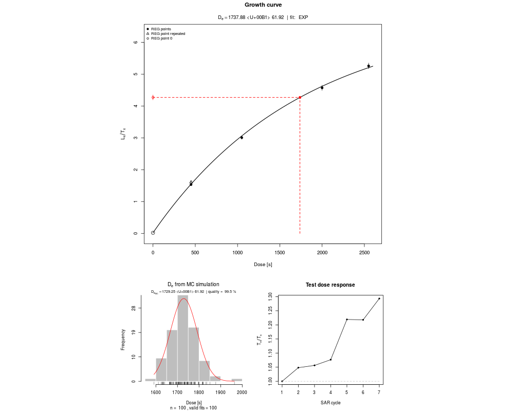
> temp <- plot_GrowthCurve(LxTxData)
[plot_GrowthCurve()] Fit: EXP | De = 1737.88 | D01 = 1766.07
> get_RLum(temp)
De De.Error D01 D01.ERROR D02 D02.ERROR De.MC Fit
1 1737.88 53.35 1766.07 85.97893 NA NA 1732.3 EXP
>
> ##(1a) to access the fitting value try
> get_RLum(temp, data.object = "Fit")
Nonlinear regression model
model: y ~ a * (1 - exp(-(x + c)/b))
data: data
a b c
6.806 1766.074 5.051
weighted residual sum-of-squares: 0.0004268
Number of iterations to convergence: 4
Achieved convergence tolerance: 1.49e-08
>
> ##(2) plot the growth curve only - uncomment to use
> ##pdf(file = "~/Desktop/Growth_Curve_Dummy.pdf", paper = "special")
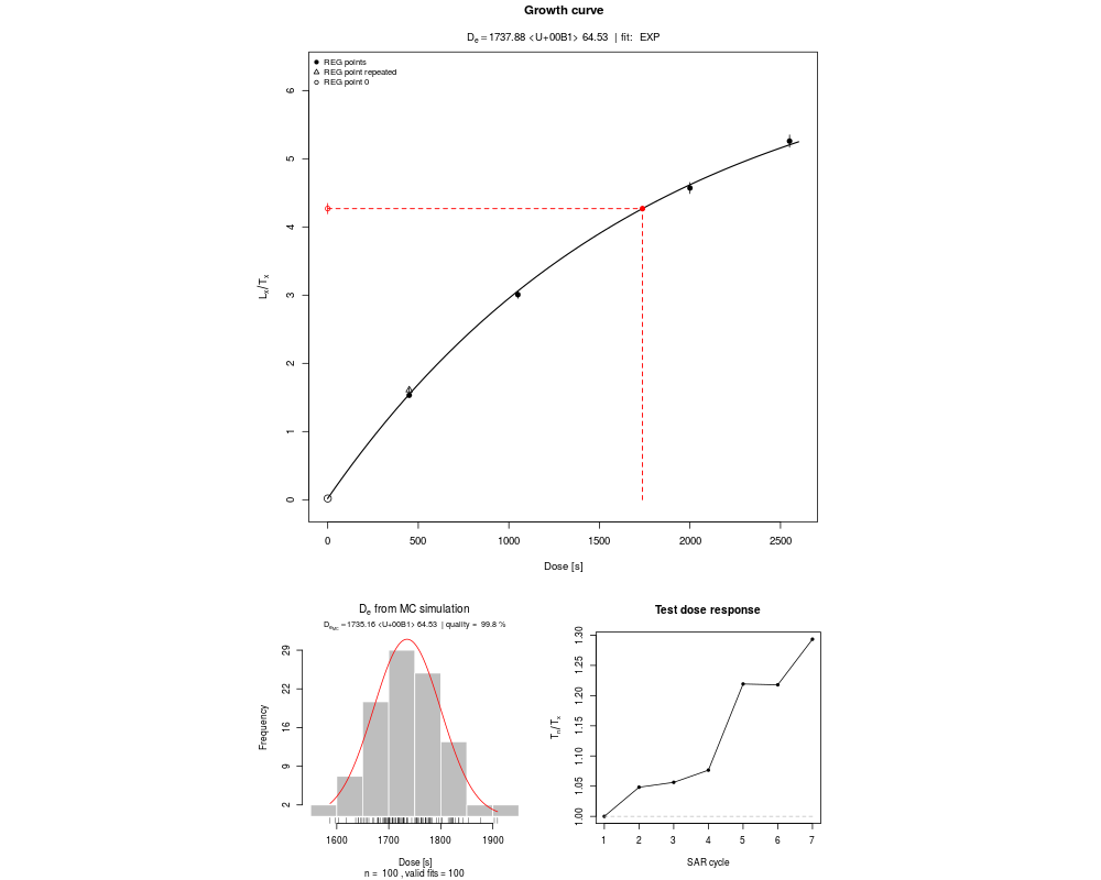
> plot_GrowthCurve(LxTxData)
[plot_GrowthCurve()] Fit: EXP | De = 1737.88 | D01 = 1766.07
> ##dev.off()
>
> ##(3) plot growth curve with pdf output - uncomment to use, single output
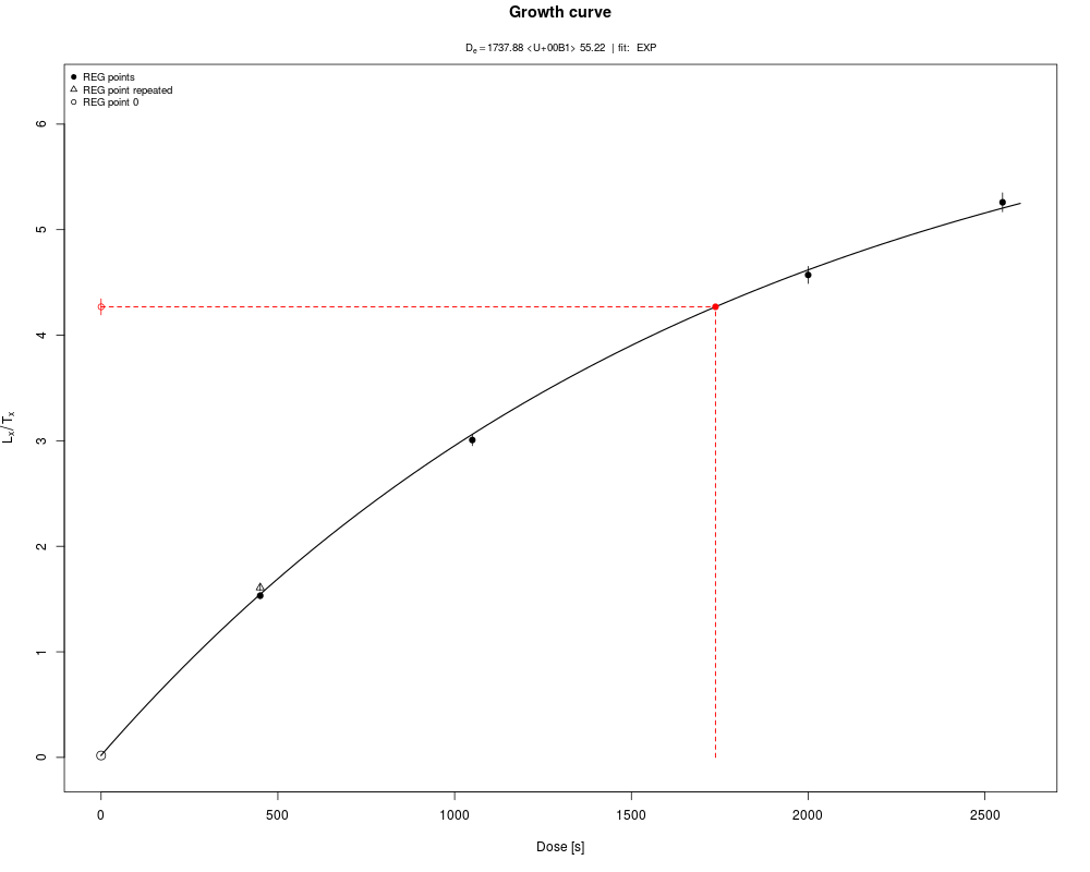
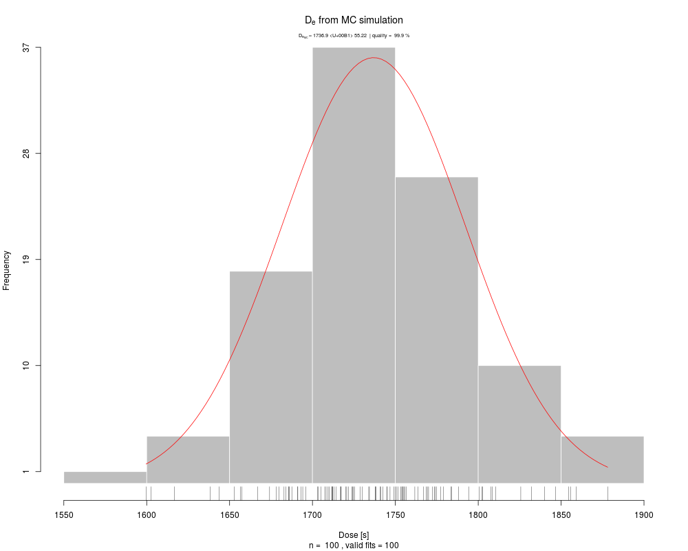
> ##pdf(file = "~/Desktop/Growth_Curve_Dummy.pdf", paper = "special")
> plot_GrowthCurve(LxTxData, output.plotExtended.single = TRUE)
[plot_GrowthCurve()] Fit: EXP | De = 1737.88 | D01 = 1766.07
> ##dev.off()
>
>
>
>
>
>
> dev.off()
null device
1
>
|