Supported by Dr. Osamu Ogasawara and  . . |
|
Last data update: 2014.03.03 |
Plot a histogram with separate error plotDescriptionFunction plots a predefined histogram with an accompanying error plot as suggested by Rex Galbraith at the UK LED in Oxford 2010. Usageplot_Histogram(data, na.rm = TRUE, mtext, cex.global, se, rug, normal_curve, summary, summary.pos, colour, interactive = FALSE, ...) Arguments
DetailsIf the normal curve is added, the y-axis in the histogram will show the
probability density. Function version0.4.4 (2016-05-19 23:47:19) NoteThe input data is not restricted to a special type. Author(s)Michael Dietze, GFZ Potsdam (Germany), See Also
Examples
## load data
data(ExampleData.DeValues, envir = environment())
ExampleData.DeValues <-
Second2Gray(ExampleData.DeValues$BT998, dose.rate = c(0.0438,0.0019))
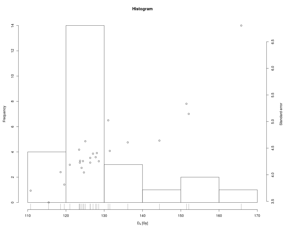
## plot histogram the easiest way
plot_Histogram(ExampleData.DeValues)
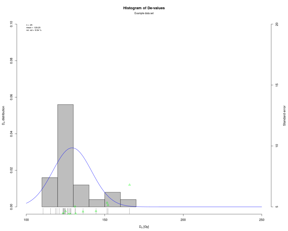
## plot histogram with some more modifications
plot_Histogram(ExampleData.DeValues,
rug = TRUE,
normal_curve = TRUE,
cex.global = 0.9,
pch = 2,
colour = c("grey", "black", "blue", "green"),
summary = c("n", "mean", "sdrel"),
summary.pos = "topleft",
main = "Histogram of De-values",
mtext = "Example data set",
ylab = c(expression(paste(D[e], " distribution")),
"Standard error"),
xlim = c(100, 250),
ylim = c(0, 0.1, 5, 20))
Results
R version 3.3.1 (2016-06-21) -- "Bug in Your Hair"
Copyright (C) 2016 The R Foundation for Statistical Computing
Platform: x86_64-pc-linux-gnu (64-bit)

R is free software and comes with ABSOLUTELY NO WARRANTY.
You are welcome to redistribute it under certain conditions.
Type 'license()' or 'licence()' for distribution details.

R is a collaborative project with many contributors.
Type 'contributors()' for more information and
'citation()' on how to cite R or R packages in publications.

Type 'demo()' for some demos, 'help()' for on-line help, or
'help.start()' for an HTML browser interface to help.
Type 'q()' to quit R.

> library(Luminescence)
Welcome to the R package Luminescence version 0.6.0 [Built: 2016-05-30 16:47:30 UTC]
The R-package Luminescence manual: 'Call unto me, and I will answer thee, and will shew thee great things, and difficult, which thou knowest not.'
> png(filename="/home/ddbj/snapshot/RGM3/R_CC/result/Luminescence/plot_Histogram.Rd_%03d_medium.png", width=480, height=480)
> ### Name: plot_Histogram
> ### Title: Plot a histogram with separate error plot
> ### Aliases: plot_Histogram
>
> ### ** Examples
>
>
> ## load data
> data(ExampleData.DeValues, envir = environment())
> ExampleData.DeValues <-
+   Second2Gray(ExampleData.DeValues$BT998, dose.rate = c(0.0438,0.0019))
>
> ## plot histogram the easiest way
> plot_Histogram(ExampleData.DeValues)
>
> ## plot histogram with some more modifications
> plot_Histogram(ExampleData.DeValues,
+                rug = TRUE,
+                normal_curve = TRUE,
+                cex.global = 0.9,
+                pch = 2,
+                colour = c("grey", "black", "blue", "green"),
+                summary = c("n", "mean", "sdrel"),
+                summary.pos = "topleft",
+                main = "Histogram of De-values",
+                mtext = "Example data set",
+                ylab = c(expression(paste(D[e], " distribution")),
+                         "Standard error"),
+                xlim = c(100, 250),
+                ylim = c(0, 0.1, 5, 20))
>
>
>
>
>
>
>
> dev.off()
null device
          1
>
|