Supported by Dr. Osamu Ogasawara and  . . |
|
Last data update: 2014.03.03 |
Function to create a Radial PlotDescriptionA Galbraith's radial plot is produced on a logarithmic or a linear scale. Usageplot_RadialPlot(data, na.rm = TRUE, negatives = "remove", log.z = TRUE, central.value, centrality = "mean.weighted", mtext, summary, summary.pos, legend, legend.pos, stats, rug = FALSE, plot.ratio, bar.col, y.ticks = TRUE, grid.col, line, line.col, line.label, output = FALSE, ...) Arguments
DetailsDetails and the theoretical background of the radial plot are given in the
cited literature. This function is based on an S script of Rex Galbraith. To
reduce the manual adjustments, the function has been rewritten. Thanks to
Rex Galbraith for useful comments on this function. Earlier versions of the Radial Plot in this package had the 2-sigma-bar
drawn onto the z-axis. However, this might have caused misunderstanding in
that the 2-sigma range may also refer to the z-scale, which it does not!
Rather it applies only to the x-y-coordinate system (standardised error vs.
precision). A spread in doses or ages must be drawn as lines originating at
zero precision (x0) and zero standardised estimate (y0). Such a range may be
drawn by adding lines to the radial plot ( A statistic summary, i.e. a collection of statistic measures of
centrality and dispersion (and further measures) can be added by specifying
one or more of the following keywords: ValueReturns a plot object. Function version0.5.3 (2016-05-19 23:47:38) Author(s)Michael Dietze, GFZ Potsdam (Germany), ReferencesGalbraith, R.F., 1988. Graphical Display of Estimates Having Differing Standard Errors. Technometrics, 30 (3), 271-281. Galbraith, R.F., 1990. The radial plot: Graphical assessment of spread in ages. International Journal of Radiation Applications and Instrumentation. Part D. Nuclear Tracks and Radiation Measurements, 17 (3), 207-214. Galbraith, R. & Green, P., 1990. Estimating the component ages in a finite mixture. International Journal of Radiation Applications and Instrumentation. Part D. Nuclear Tracks and Radiation Measurements, 17 (3) 197-206. Galbraith, R.F. & Laslett, G.M., 1993. Statistical models for mixed fission track ages. Nuclear Tracks And Radiation Measurements, 21 (4), 459-470. Galbraith, R.F., 1994. Some Applications of Radial Plots. Journal of the American Statistical Association, 89 (428), 1232-1242. Galbraith, R.F., 2010. On plotting OSL equivalent doses. Ancient TL, 28 (1), 1-10. Galbraith, R.F. & Roberts, R.G., 2012. Statistical aspects of equivalent dose and error calculation and display in OSL dating: An overview and some recommendations. Quaternary Geochronology, 11, 1-27. See Also
Examples
## load example data
data(ExampleData.DeValues, envir = environment())
ExampleData.DeValues <- Second2Gray(ExampleData.DeValues$BT998, c(0.0438,0.0019))
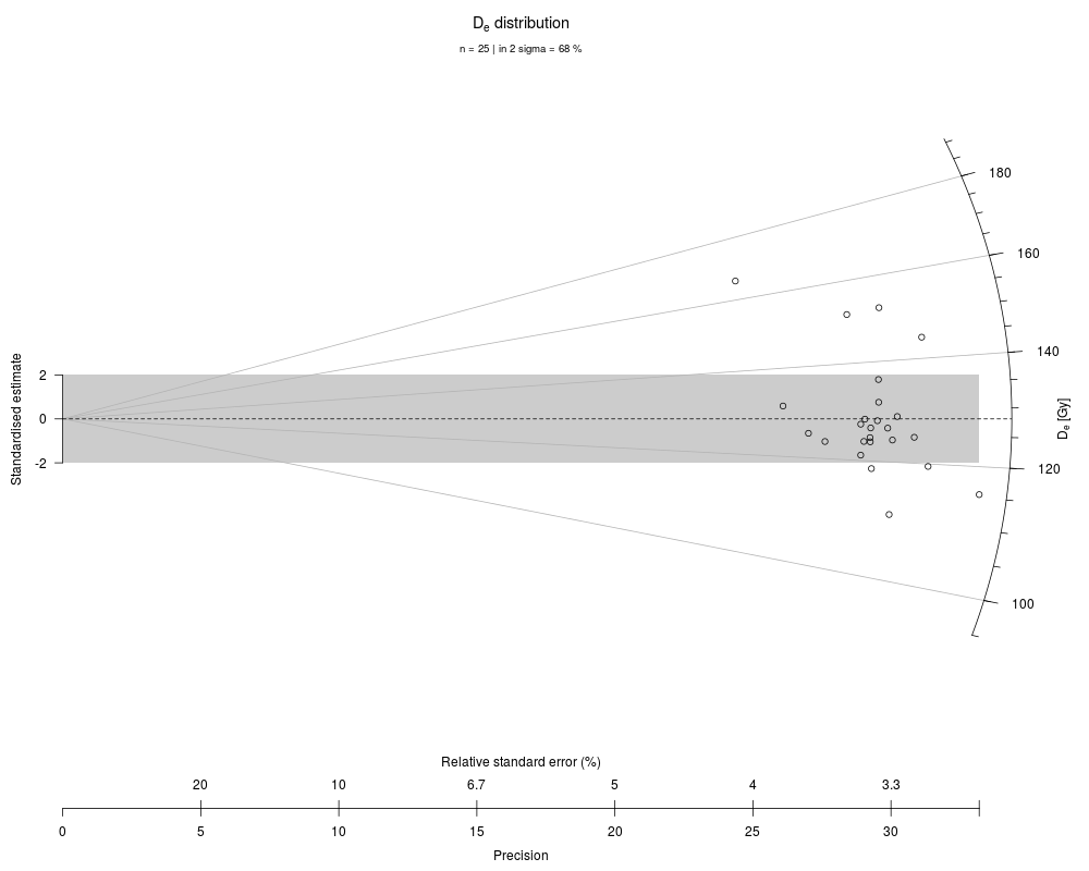
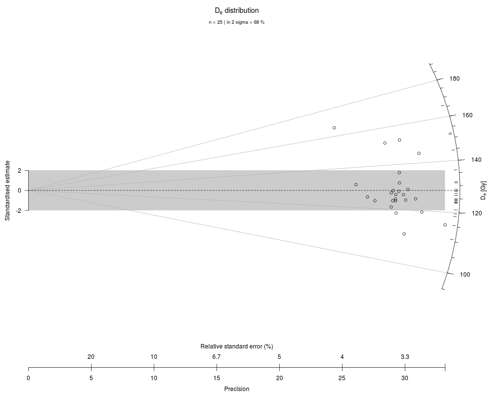
## plot the example data straightforward
plot_RadialPlot(data = ExampleData.DeValues)
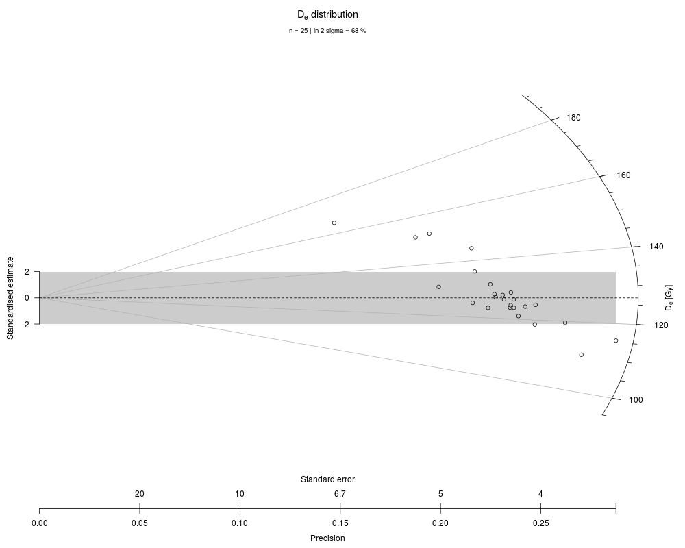
## now with linear z-scale
plot_RadialPlot(data = ExampleData.DeValues,
log.z = FALSE)
## now with output of the plot parameters
plot1 <- plot_RadialPlot(data = ExampleData.DeValues,
log.z = FALSE,
output = TRUE)
plot1
plot1$zlim
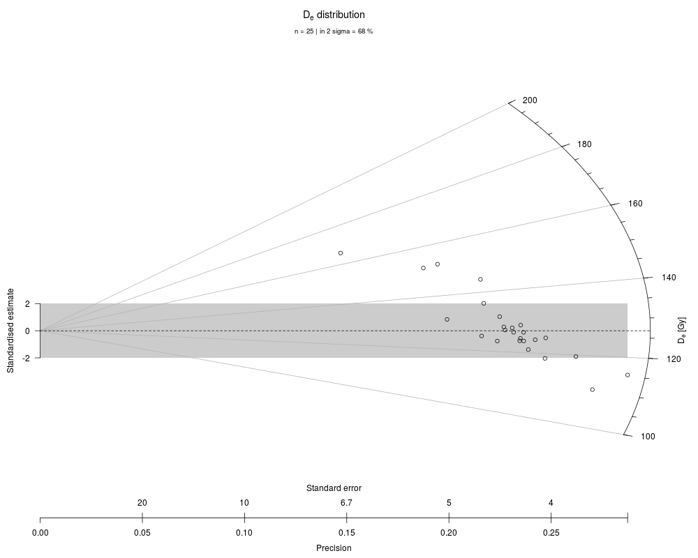
## now with adjusted z-scale limits
plot_RadialPlot(data = ExampleData.DeValues,
log.z = FALSE,
zlim = c(100, 200))
## now the two plots with serious but seasonally changing fun
#plot_RadialPlot(data = data.3, fun = TRUE)
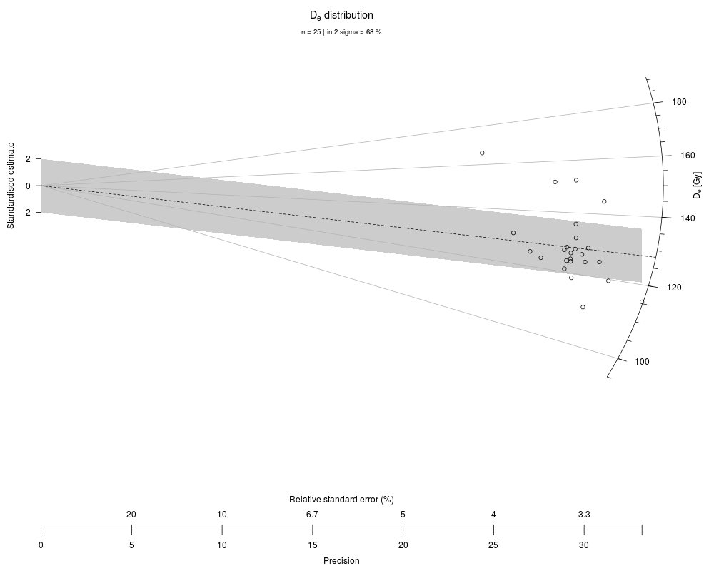
## now with user-defined central value, in log-scale again
plot_RadialPlot(data = ExampleData.DeValues,
central.value = 150)
## now with a rug, indicating individual De values at the z-scale
plot_RadialPlot(data = ExampleData.DeValues,
rug = TRUE)
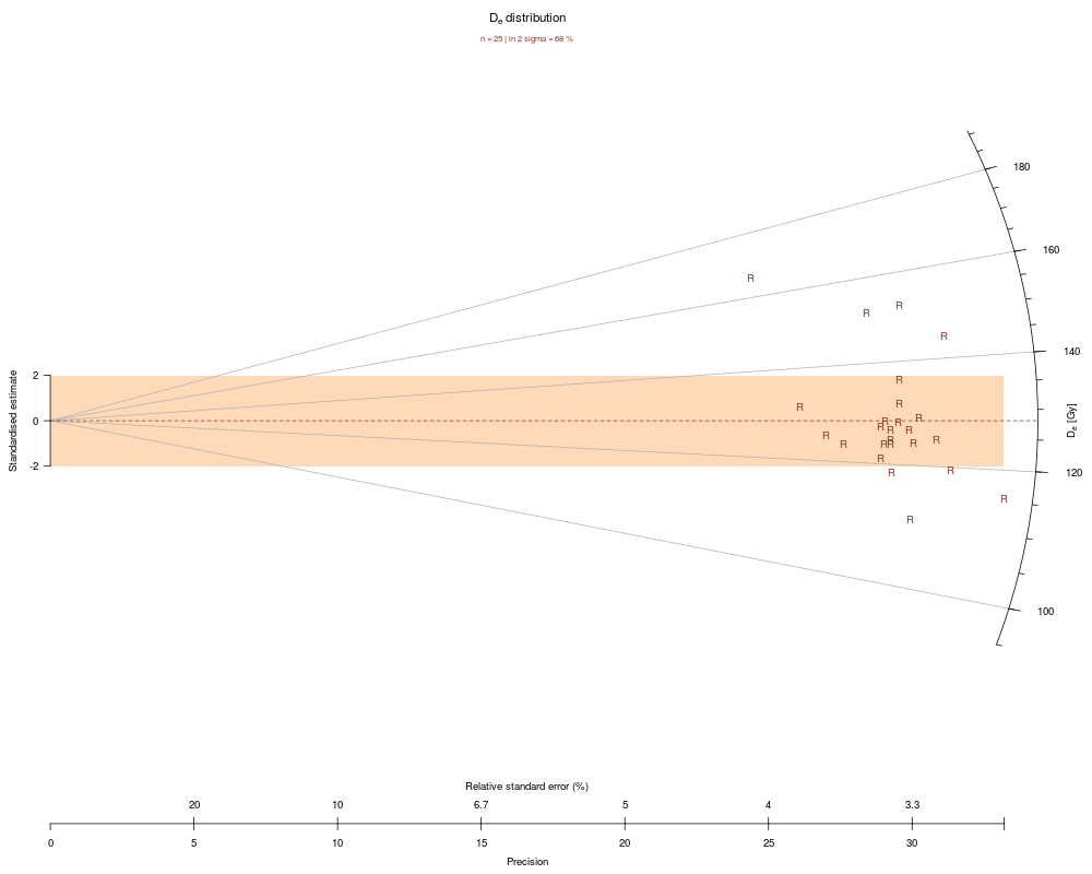
## now with legend, colour, different points and smaller scale
plot_RadialPlot(data = ExampleData.DeValues,
legend.text = "Sample 1",
col = "tomato4",
bar.col = "peachpuff",
pch = "R",
cex = 0.8)
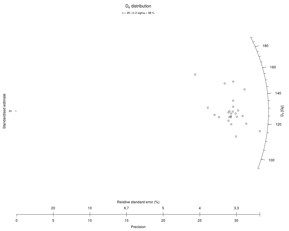
## now without 2-sigma bar, y-axis, grid lines and central value line
plot_RadialPlot(data = ExampleData.DeValues,
bar.col = "none",
grid.col = "none",
y.ticks = FALSE,
lwd = 0)
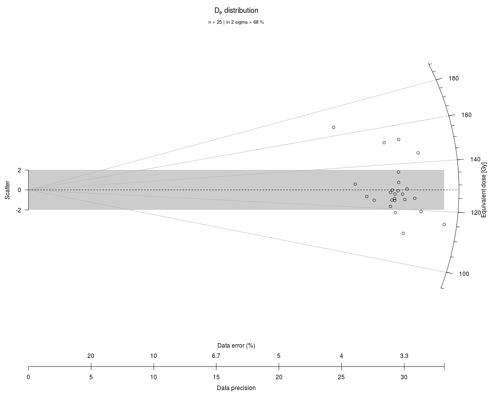
## now with user-defined axes labels
plot_RadialPlot(data = ExampleData.DeValues,
xlab = c("Data error (%)",
"Data precision"),
ylab = "Scatter",
zlab = "Equivalent dose [Gy]")
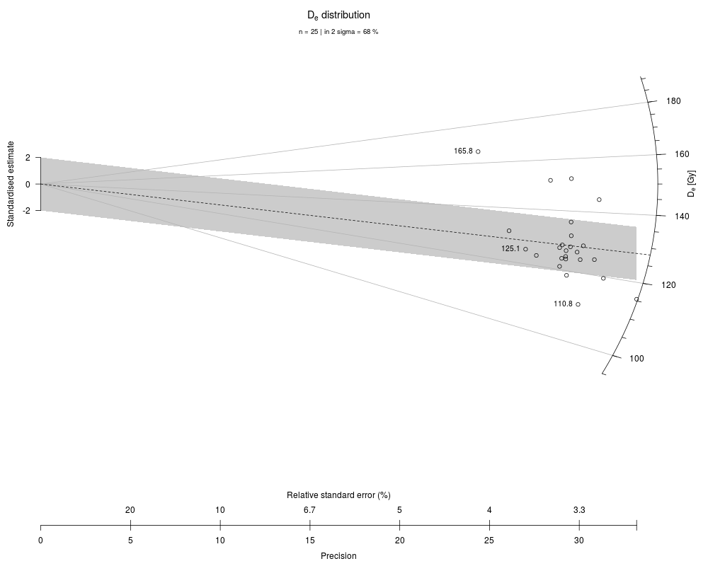
## now with minimum, maximum and median value indicated
plot_RadialPlot(data = ExampleData.DeValues,
central.value = 150,
stats = c("min", "max", "median"))
## now with a brief statistical summary
plot_RadialPlot(data = ExampleData.DeValues,
summary = c("n", "in.2s"))
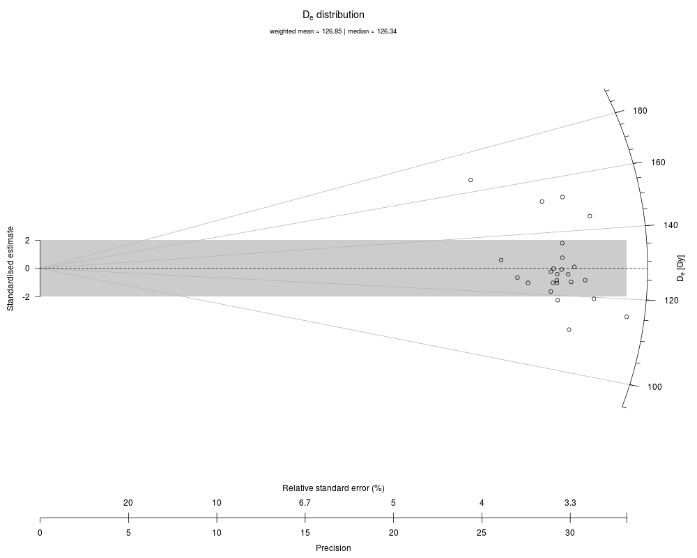
## now with another statistical summary as subheader
plot_RadialPlot(data = ExampleData.DeValues,
summary = c("mean.weighted", "median"),
summary.pos = "sub")
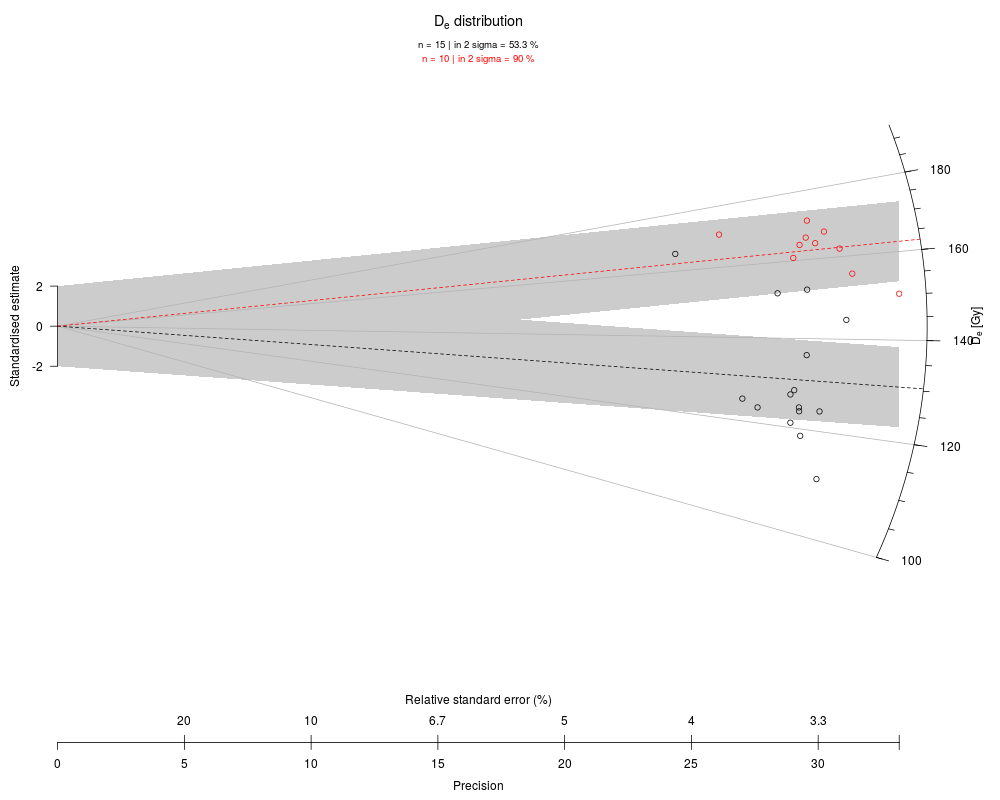
## now the data set is split into sub-groups, one is manipulated
data.1 <- ExampleData.DeValues[1:15,]
data.2 <- ExampleData.DeValues[16:25,] * 1.3
## now a common dataset is created from the two subgroups
data.3 <- list(data.1, data.2)
## now the two data sets are plotted in one plot
plot_RadialPlot(data = data.3)
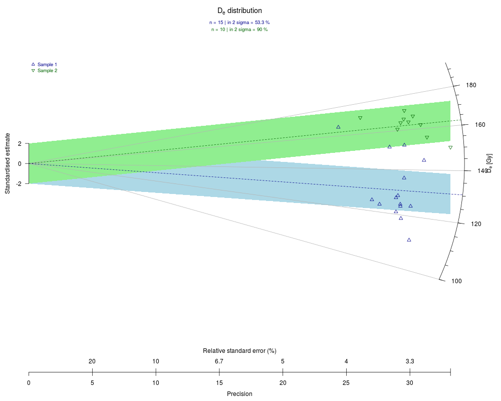
## now with some graphical modification
plot_RadialPlot(data = data.3,
col = c("darkblue", "darkgreen"),
bar.col = c("lightblue", "lightgreen"),
pch = c(2, 6),
summary = c("n", "in.2s"),
summary.pos = "sub",
legend = c("Sample 1", "Sample 2"))
Results
R version 3.3.1 (2016-06-21) -- "Bug in Your Hair"
Copyright (C) 2016 The R Foundation for Statistical Computing
Platform: x86_64-pc-linux-gnu (64-bit)

R is free software and comes with ABSOLUTELY NO WARRANTY.
You are welcome to redistribute it under certain conditions.
Type 'license()' or 'licence()' for distribution details.

R is a collaborative project with many contributors.
Type 'contributors()' for more information and
'citation()' on how to cite R or R packages in publications.

Type 'demo()' for some demos, 'help()' for on-line help, or
'help.start()' for an HTML browser interface to help.
Type 'q()' to quit R.

> library(Luminescence)
Welcome to the R package Luminescence version 0.6.0 [Built: 2016-05-30 16:47:30 UTC]
Rubber mallet to steel cylinder: 'Let's rock and roll.'
> png(filename="/home/ddbj/snapshot/RGM3/R_CC/result/Luminescence/plot_RadialPlot.Rd_%03d_medium.png", width=480, height=480)
> ### Name: plot_RadialPlot
> ### Title: Function to create a Radial Plot
> ### Aliases: plot_RadialPlot
>
> ### ** Examples
>
>
> ## load example data
> data(ExampleData.DeValues, envir = environment())
> ExampleData.DeValues <- Second2Gray(ExampleData.DeValues$BT998, c(0.0438,0.0019))
>
> ## plot the example data straightforward
> plot_RadialPlot(data = ExampleData.DeValues)
>
> ## now with linear z-scale
> plot_RadialPlot(data = ExampleData.DeValues,
+                 log.z = FALSE)
>
> ## now with output of the plot parameters
> plot1 <- plot_RadialPlot(data = ExampleData.DeValues,
+                          log.z = FALSE,
+                          output = TRUE)
> plot1
$data
$data[[1]]
       De error      z    se z.central precision std.estimate std.estimate.plot
1  151.48 5.334 151.48 5.334  126.8469 0.1874766   4.61813168        4.61813168
2  152.08 5.144 152.08 5.144  126.8469 0.1944012   4.90534883        4.90534883
3  165.80 6.805 165.80 6.805  126.8469 0.1469508   5.72419021        5.72419021
4  136.15 4.608 136.15 4.608  126.8469 0.2170139   2.01890503        2.01890503
5  144.42 4.642 144.42 4.642  126.8469 0.2154244   3.78567738        3.78567738
6  123.44 4.471 123.44 4.471  126.8469 0.2236636  -0.76199634       -0.76199634
7  123.64 4.227 123.64 4.227  126.8469 0.2365744  -0.75866705       -0.75866705
8  127.07 4.396 127.07 4.396  126.8469 0.2274795   0.05075395        0.05075395
9  125.06 4.630 125.06 4.630  126.8469 0.2159827  -0.38593642       -0.38593642
10 124.45 4.256 124.45 4.256  126.8469 0.2349624  -0.56317801       -0.56317801
11 118.60 4.049 118.60 4.049  126.8469 0.2469746  -2.03677096       -2.03677096
12 128.08 4.408 128.08 4.408  126.8469 0.2268603   0.27974464        0.27974464
13 110.78 3.701 110.78 3.701  126.8469 0.2701972  -4.34122821       -4.34122821
14 121.02 4.187 121.02 4.187  126.8469 0.2388345  -1.39166124       -1.39166124
15 124.09 4.129 124.09 4.129  126.8469 0.2421894  -0.66768845       -0.66768845
16 124.70 4.043 124.70 4.043  126.8469 0.2473411  -0.53101302       -0.53101302
17 123.68 4.262 123.68 4.262  126.8469 0.2346316  -0.74305153       -0.74305153
18 126.34 4.228 126.34 4.228  126.8469 0.2365184  -0.11988780       -0.11988780
19 128.59 4.254 128.59 4.254  126.8469 0.2350729   0.40975890        0.40975890
20 131.46 4.448 131.46 4.448  126.8469 0.2248201   1.03712104        1.03712104
21 127.77 4.330 127.77 4.330  126.8469 0.2309469   0.21319039        0.21319039
22 131.05 5.023 131.05 5.023  126.8469 0.1990842   0.83677372        0.83677372
23 126.34 4.317 126.34 4.317  126.8469 0.2316423  -0.11741617       -0.11741617
24 115.49 3.479 115.49 3.479  126.8469 0.2874389  -3.26441093       -3.26441093
25 119.58 3.815 119.58 3.815  126.8469 0.2621232  -1.90481930       -1.90481930


$data.global
       De error      z    se z.central precision std.estimate std.estimate.plot
1  151.48 5.334 151.48 5.334  126.8469 0.1874766   4.61813168        4.61813168
2  152.08 5.144 152.08 5.144  126.8469 0.1944012   4.90534883        4.90534883
3  165.80 6.805 165.80 6.805  126.8469 0.1469508   5.72419021        5.72419021
4  136.15 4.608 136.15 4.608  126.8469 0.2170139   2.01890503        2.01890503
5  144.42 4.642 144.42 4.642  126.8469 0.2154244   3.78567738        3.78567738
6  123.44 4.471 123.44 4.471  126.8469 0.2236636  -0.76199634       -0.76199634
7  123.64 4.227 123.64 4.227  126.8469 0.2365744  -0.75866705       -0.75866705
8  127.07 4.396 127.07 4.396  126.8469 0.2274795   0.05075395        0.05075395
9  125.06 4.630 125.06 4.630  126.8469 0.2159827  -0.38593642       -0.38593642
10 124.45 4.256 124.45 4.256  126.8469 0.2349624  -0.56317801       -0.56317801
11 118.60 4.049 118.60 4.049  126.8469 0.2469746  -2.03677096       -2.03677096
12 128.08 4.408 128.08 4.408  126.8469 0.2268603   0.27974464        0.27974464
13 110.78 3.701 110.78 3.701  126.8469 0.2701972  -4.34122821       -4.34122821
14 121.02 4.187 121.02 4.187  126.8469 0.2388345  -1.39166124       -1.39166124
15 124.09 4.129 124.09 4.129  126.8469 0.2421894  -0.66768845       -0.66768845
16 124.70 4.043 124.70 4.043  126.8469 0.2473411  -0.53101302       -0.53101302
17 123.68 4.262 123.68 4.262  126.8469 0.2346316  -0.74305153       -0.74305153
18 126.34 4.228 126.34 4.228  126.8469 0.2365184  -0.11988780       -0.11988780
19 128.59 4.254 128.59 4.254  126.8469 0.2350729   0.40975890        0.40975890
20 131.46 4.448 131.46 4.448  126.8469 0.2248201   1.03712104        1.03712104
21 127.77 4.330 127.77 4.330  126.8469 0.2309469   0.21319039        0.21319039
22 131.05 5.023 131.05 5.023  126.8469 0.1990842   0.83677372        0.83677372
23 126.34 4.317 126.34 4.317  126.8469 0.2316423  -0.11741617       -0.11741617
24 115.49 3.479 115.49 3.479  126.8469 0.2874389  -3.26441093       -3.26441093
25 119.58 3.815 119.58 3.815  126.8469 0.2621232  -1.90481930       -1.90481930
   NA
1   1
2   1
3   1
4   1
5   1
6   1
7   1
8   1
9   1
10  1
11  1
12  1
13  1
14  1
15  1
16  1
17  1
18  1
19  1
20  1
21  1
22  1
23  1
24  1
25  1

$xlim
[1] 0.0000000 0.2874389

$ylim
[1] -16.08311  20.09820

$zlim
[1]  93.89862 191.06569

$r
[1] 0.2985416

$plot.ratio
[1] 0.8181818

$ticks.major
     tick.x1.major tick.x2.major tick.y1.major tick.y2.major
[1,]     0.2854285     0.2897099     -7.662866     -7.777809
[2,]     0.2976332     0.3020977     -2.037860     -2.068428
[3,]     0.2952298     0.2996582      3.883191      3.941439
[4,]     0.2792013     0.2833893      9.256392      9.395238
[5,]     0.2552062     0.2590343     13.565004     13.768479

$ticks.minor
      tick.x1.minor tick.x2.minor tick.y1.minor tick.y2.minor
 [1,]     0.2805631     0.2825271    -8.9350621    -8.9976075
 [2,]     0.2854285     0.2874265    -7.6628657    -7.7165057
 [3,]     0.2896629     0.2916905    -6.3282319    -6.3725295
 [4,]     0.2931655     0.2952176    -4.9389249    -4.9734974
 [5,]     0.2958465     0.2979174    -3.5048592    -3.5293932
 [6,]     0.2976332     0.2997166    -2.0378605    -2.0521255
 [7,]     0.2984753     0.3005646    -0.5512497    -0.5551084
 [8,]     0.2983483     0.3004367     0.9407262     0.9473113
 [9,]     0.2972560     0.2993368     2.4235620     2.4405269
[10,]     0.2952298     0.2972964     3.8831908     3.9103731
[11,]     0.2923263     0.2943726     5.3066331     5.3437795
[12,]     0.2886233     0.2906437     6.6825291     6.7293069
[13,]     0.2842141     0.2862035     8.0015107     8.0575213
[14,]     0.2792013     0.2811557     9.2563922     9.3211869
[15,]     0.2736917     0.2756075    10.4421902    10.5152856
[16,]     0.2677906     0.2696652    11.5560001    11.6368921
[17,]     0.2615982     0.2634294    12.5967683    12.6849456
[18,]     0.2552062     0.2569926    13.5650040    13.6599591
[19,]     0.2486964     0.2504372    14.4624680    14.5637053
[20,]     0.2421396     0.2438345    15.2918668    15.3989099

$labels
       label.x   label.y label.z.text
[1,] 0.2939913 -7.777809          100
[2,] 0.3065622 -2.068428          120
[3,] 0.3040867  3.941439          140
[4,] 0.2875773  9.395238          160
[5,] 0.2628624 13.768479          180

$polygons
     [,1] [,2]      [,3]      [,4] [,5] [,6] [,7] [,8]
[1,]    0    0 0.2874389 0.2874389   -2    2    2   -2

$ellipse.lims
           [,1]       [,2]
[1,]  0.2407419  0.2985415
[2,] -8.9350621 15.4601557

> plot1$zlim
[1]  93.89862 191.06569
>
> ## now with adjusted z-scale limits
> plot_RadialPlot(data = ExampleData.DeValues,
+                log.z = FALSE,
+                zlim = c(100, 200))
>
> ## now the two plots with serious but seasonally changing fun
> #plot_RadialPlot(data = data.3, fun = TRUE)
>
> ## now with user-defined central value, in log-scale again
> plot_RadialPlot(data = ExampleData.DeValues,
+                 central.value = 150)
>
> ## now with a rug, indicating individual De values at the z-scale
> plot_RadialPlot(data = ExampleData.DeValues,
+                 rug = TRUE)
>
> ## now with legend, colour, different points and smaller scale
> plot_RadialPlot(data = ExampleData.DeValues,
+                 legend.text = "Sample 1",
+                 col = "tomato4",
+                 bar.col = "peachpuff",
+                 pch = "R",
+                 cex = 0.8)
>
> ## now without 2-sigma bar, y-axis, grid lines and central value line
> plot_RadialPlot(data = ExampleData.DeValues,
+                 bar.col = "none",
+                 grid.col = "none",
+                 y.ticks = FALSE,
+                 lwd = 0)
>
> ## now with user-defined axes labels
> plot_RadialPlot(data = ExampleData.DeValues,
+                 xlab = c("Data error (%)",
+                          "Data precision"),
+                 ylab = "Scatter",
+                 zlab = "Equivalent dose [Gy]")
>
> ## now with minimum, maximum and median value indicated
> plot_RadialPlot(data = ExampleData.DeValues,
+                 central.value = 150,
+                 stats = c("min", "max", "median"))
>
> ## now with a brief statistical summary
> plot_RadialPlot(data = ExampleData.DeValues,
+                 summary = c("n", "in.2s"))
>
> ## now with another statistical summary as subheader
> plot_RadialPlot(data = ExampleData.DeValues,
+                 summary = c("mean.weighted", "median"),
+                 summary.pos = "sub")
>
> ## now the data set is split into sub-groups, one is manipulated
> data.1 <- ExampleData.DeValues[1:15,]
> data.2 <- ExampleData.DeValues[16:25,] * 1.3
>
> ## now a common dataset is created from the two subgroups
> data.3 <- list(data.1, data.2)
>
> ## now the two data sets are plotted in one plot
> plot_RadialPlot(data = data.3)
>
> ## now with some graphical modification
> plot_RadialPlot(data = data.3,
+                 col = c("darkblue", "darkgreen"),
+                 bar.col = c("lightblue", "lightgreen"),
+                 pch = c(2, 6),
+                 summary = c("n", "in.2s"),
+                 summary.pos = "sub",
+                 legend = c("Sample 1", "Sample 2"))
>
>
>
>
>
>
> dev.off()
null device
          1
>
|