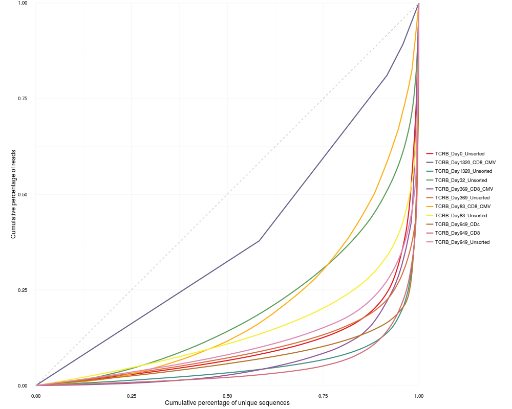
Lorenz curve

Description

Plots a Lorenz curve derived from the frequency of the amino acid sequences.

Usage

lorenzCurve(samples, list)

Arguments

Details

The Gini coefficient is an alternative metric used to calculate repertoire diversity and is derived from the Lorenz curve. The Lorenz curve is drawn such that x-axis represents the cumulative percentage of unique sequences and the y-axis represents the cumulative percentage of reads. A line passing through the origin with a slope of 1 reflects equal frequencies of all sequences. The Gini coefficient is the ratio of the area between the line of equality and the observed Lorenz curve over the total area under the line of equality.

The plot is made using the package ggplot2 and can be reformatted using ggplot2 functions. See examples below.

Value

Returns a Lorenz curve.

See Also

An excellent resource for examples on how to reformat a ggplot can be found in the R Graphics Cookbook online (http://www.cookbook-r.com/Graphs/).

Examples

file.path <- system.file("extdata", "TCRB_sequencing", package = "LymphoSeq")

file.list <- readImmunoSeq(path = file.path)

lorenzCurve(samples = names(file.list), list = file.list)

productive.aa <- productiveSeq(file.list = file.list, aggregate = "aminoAcid")

lorenzCurve(samples = names(productive.aa), list = productive.aa)

# Change the legend labels, line colors, and add a title
samples <- c("TCRB_Day0_Unsorted", "TCRB_Day32_Unsorted", 
   "TCRB_Day83_Unsorted", "TCRB_Day949_Unsorted", "TCRB_Day1320_Unsorted")

lorenz.curve <- lorenzCurve(samples = samples, list = productive.aa)

labels <- c("Day 0", "Day 32", "Day 83", "Day 949", "Day 1320")

colors <- c("navyblue", "red", "darkgreen", "orange", "purple")

lorenz.curve + ggplot2::scale_color_manual(name = "Samples", breaks = samples, 
   labels = labels, values = colors) + ggplot2::ggtitle("Figure Title")

Results

R version 3.3.1 (2016-06-21) -- "Bug in Your Hair"
Copyright (C) 2016 The R Foundation for Statistical Computing
Platform: x86_64-pc-linux-gnu (64-bit)

R is free software and comes with ABSOLUTELY NO WARRANTY.
You are welcome to redistribute it under certain conditions.
Type 'license()' or 'licence()' for distribution details.

R is a collaborative project with many contributors.
Type 'contributors()' for more information and
'citation()' on how to cite R or R packages in publications.

Type 'demo()' for some demos, 'help()' for on-line help, or
'help.start()' for an HTML browser interface to help.
Type 'q()' to quit R.

> library(LymphoSeq)
Loading required package: LymphoSeqDB
> png(filename="/home/ddbj/snapshot/RGM3/R_BC/result/LymphoSeq/lorenzCurve.Rd_%03d_medium.png", width=480, height=480)
> ### Name: lorenzCurve
> ### Title: Lorenz curve
> ### Aliases: lorenzCurve
> 
> ### ** Examples
> 
> file.path <- system.file("extdata", "TCRB_sequencing", package = "LymphoSeq")
> 
> file.list <- readImmunoSeq(path = file.path)
   |                                                                               |                                                                      |   0%   |                                                                               |======                                                                |   9%   |                                                                               |=============                                                         |  18%   |                                                                               |===================                                                   |  27%   |                                                                               |=========================                                             |  36%   |                                                                               |================================                                      |  45%   |                                                                               |======================================                                |  55%   |                                                                               |=============================================                         |  64%   |                                                                               |===================================================                   |  73%   |                                                                               |=========================================================             |  82%   |                                                                               |================================================================      |  91%   |                                                                               |======================================================================| 100%
> 
> lorenzCurve(samples = names(file.list), list = file.list)
> 
> productive.aa <- productiveSeq(file.list = file.list, aggregate = "aminoAcid")
   |                                                                               |                                                                      |   0%   |                                                                               |======                                                                |   9%   |                                                                               |=============                                                         |  18%   |                                                                               |===================                                                   |  27%   |                                                                               |=========================                                             |  36%   |                                                                               |================================                                      |  45%   |                                                                               |======================================                                |  55%   |                                                                               |=============================================                         |  64%   |                                                                               |===================================================                   |  73%   |                                                                               |=========================================================             |  82%   |                                                                               |================================================================      |  91%   |                                                                               |======================================================================| 100%
> 
> lorenzCurve(samples = names(productive.aa), list = productive.aa)
> 
> # Change the legend labels, line colors, and add a title
> samples <- c("TCRB_Day0_Unsorted", "TCRB_Day32_Unsorted", 
+    "TCRB_Day83_Unsorted", "TCRB_Day949_Unsorted", "TCRB_Day1320_Unsorted")
> 
> lorenz.curve <- lorenzCurve(samples = samples, list = productive.aa)
> 
> labels <- c("Day 0", "Day 32", "Day 83", "Day 949", "Day 1320")
> 
> colors <- c("navyblue", "red", "darkgreen", "orange", "purple")
> 
> lorenz.curve + ggplot2::scale_color_manual(name = "Samples", breaks = samples, 
+    labels = labels, values = colors) + ggplot2::ggtitle("Figure Title")
Scale for 'colour' is already present. Adding another scale for 'colour',
which will replace the existing scale.
> 
> 
> 
> 
> 
> dev.off()
null device 
          1 
>