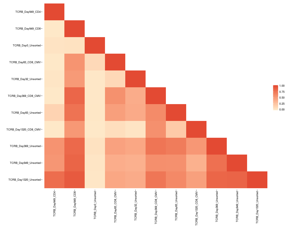
Pairwise comparison plot

Description

Creates a heat map from a similarity or Bhattacharyya matrix.

Usage

pairwisePlot(matrix)

Arguments

Details

The plot is made using the package ggplot2 and can be reformatted using ggplot2 functions. See examples below.

Value

A pairwise comparison heat map.

See Also

An excellent resource for examples on how to reformat a ggplot can be found in the R Graphics Cookbook online (http://www.cookbook-r.com/Graphs/). The functions to create the similarity or Bhattacharyya matrix can be found here: similarityMatrix and bhattacharyyaMatrix

Examples

file.path <- system.file("extdata", "TCRB_sequencing", package = "LymphoSeq")

file.list <- readImmunoSeq(path = file.path)

productive.aa <- productiveSeq(file.list = file.list, aggregate = "aminoAcid")

similarity.matrix <- similarityMatrix(productive.seqs = productive.aa)

pairwisePlot(matrix = similarity.matrix)

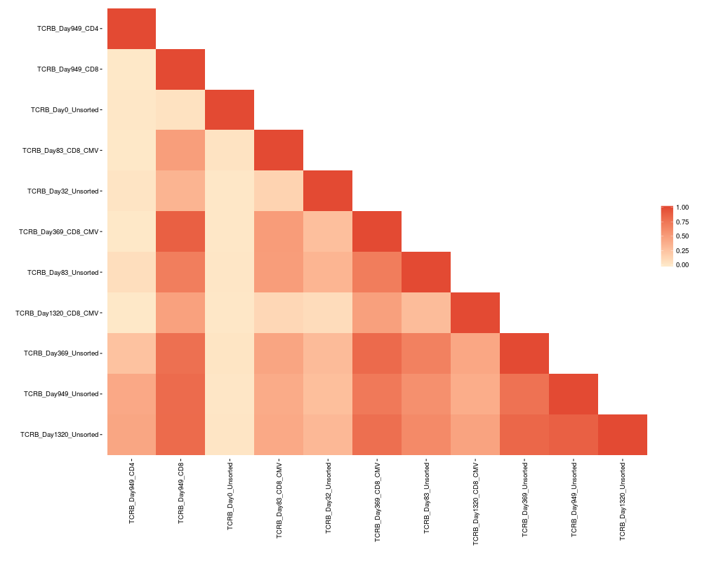
bhattacharyya.matrix <- bhattacharyyaMatrix(productive.seqs = productive.aa)

pairwisePlot(matrix = bhattacharyya.matrix)

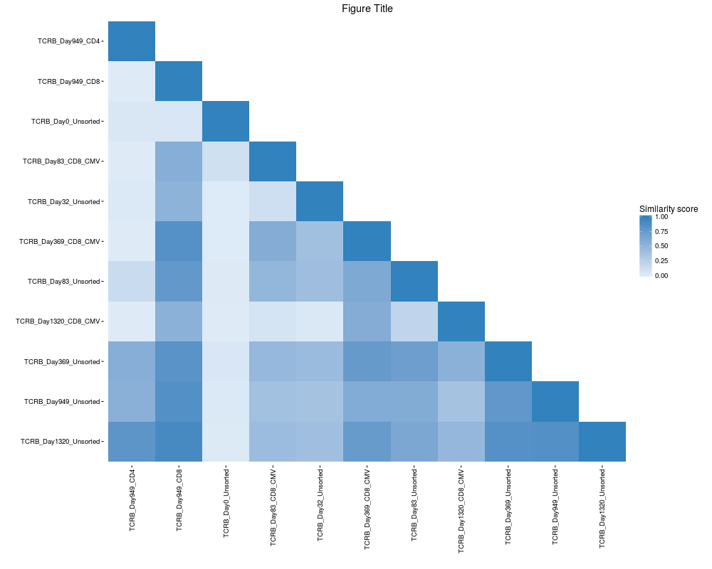
# Change plot color, title legend, and add title
pairwisePlot(matrix = similarity.matrix) + 
   ggplot2::scale_fill_gradient(low = "#deebf7", high = "#3182bd") + 
   ggplot2::labs(fill = "Similarity score") + ggplot2::ggtitle("Figure Title")

Results

R version 3.3.1 (2016-06-21) -- "Bug in Your Hair"
Copyright (C) 2016 The R Foundation for Statistical Computing
Platform: x86_64-pc-linux-gnu (64-bit)

R is free software and comes with ABSOLUTELY NO WARRANTY.
You are welcome to redistribute it under certain conditions.
Type 'license()' or 'licence()' for distribution details.

R is a collaborative project with many contributors.
Type 'contributors()' for more information and
'citation()' on how to cite R or R packages in publications.

Type 'demo()' for some demos, 'help()' for on-line help, or
'help.start()' for an HTML browser interface to help.
Type 'q()' to quit R.

> library(LymphoSeq)
Loading required package: LymphoSeqDB
> png(filename="/home/ddbj/snapshot/RGM3/R_BC/result/LymphoSeq/pairwisePlot.Rd_%03d_medium.png", width=480, height=480)
> ### Name: pairwisePlot
> ### Title: Pairwise comparison plot
> ### Aliases: pairwisePlot
> 
> ### ** Examples
> 
> file.path <- system.file("extdata", "TCRB_sequencing", package = "LymphoSeq")
> 
> file.list <- readImmunoSeq(path = file.path)
   |                                                                               |                                                                      |   0%   |                                                                               |======                                                                |   9%   |                                                                               |=============                                                         |  18%   |                                                                               |===================                                                   |  27%   |                                                                               |=========================                                             |  36%   |                                                                               |================================                                      |  45%   |                                                                               |======================================                                |  55%   |                                                                               |=============================================                         |  64%   |                                                                               |===================================================                   |  73%   |                                                                               |=========================================================             |  82%   |                                                                               |================================================================      |  91%   |                                                                               |======================================================================| 100%
> 
> productive.aa <- productiveSeq(file.list = file.list, aggregate = "aminoAcid")
   |                                                                               |                                                                      |   0%   |                                                                               |======                                                                |   9%   |                                                                               |=============                                                         |  18%   |                                                                               |===================                                                   |  27%   |                                                                               |=========================                                             |  36%   |                                                                               |================================                                      |  45%   |                                                                               |======================================                                |  55%   |                                                                               |=============================================                         |  64%   |                                                                               |===================================================                   |  73%   |                                                                               |=========================================================             |  82%   |                                                                               |================================================================      |  91%   |                                                                               |======================================================================| 100%
> 
> similarity.matrix <- similarityMatrix(productive.seqs = productive.aa)
> 
> pairwisePlot(matrix = similarity.matrix)
> 
> bhattacharyya.matrix <- bhattacharyyaMatrix(productive.seqs = productive.aa)
> 
> pairwisePlot(matrix = bhattacharyya.matrix)
> 
> # Change plot color, title legend, and add title
> pairwisePlot(matrix = similarity.matrix) + 
+    ggplot2::scale_fill_gradient(low = "#deebf7", high = "#3182bd") + 
+    ggplot2::labs(fill = "Similarity score") + ggplot2::ggtitle("Figure Title")
Scale for 'fill' is already present. Adding another scale for 'fill', which
will replace the existing scale.
> 
> 
> 
> 
> 
> dev.off()
null device 
          1 
>