R Graphical Manual

Browse All

Last data update: 2014.03.03

R: Get map lines in the model projection units

get.map.lines.M3.proj

R Documentation

Get map lines in the model projection units

Description

Get map lines in the model projection units.

Usage

get.map.lines.M3.proj(file, database = "state", units, ...)

Arguments

`file`	File name of Models3-formatted file providing the model projection.
`database`	Geographical database to use. Choices include “state” (default), “world”, “worldHires”, “canusamex”, etc. Use “canusamex” to get the national boundaries of the Canada, the USA, and Mexico, along with the boundaries of the states. The other choices (“state”, “world”, etc.) are the names of databases included with the maps and mapdata packages. (See the `map` function.) Default is “state”.
`units`	Units for coordinates of grid rows or columns. Must be one of “m”, “km”, or “deg”. If unspecified, the default is “deg” if the file has a longitude/latitude grid, and “km” otherwise.
`...`	Other arguments to pass to `get.proj.info.M3` function. In this case, the only relevant argument would be the earth radius to use for the projection in `file`.

Details

This function depends on the maps and mapdata packages to get the appropriate map boundary lines (for states, countries, etc.), ncdf4 to read the projection information from the Models3-formatted file (using a call to function get.proj.info.M3), and rgdal (which is an interface to GDAL (Geospatial Data Abstraction Library, http://www.gdal.org) to project the boundary lines to the specified projection.

Value

Map lines for the projection described in file in either kilometers or meters (depending on value of units.km). This is a matrix, with x-coordinates in the first column and y-coordinates in the second column.

Warning

This function will only work with Lambert conic conformal or polar stereographic projections.

Author(s)

Jenise Swall

References

http://www.gdal.org

Examples

## Find the path to the demo file.
polar.file <- system.file("extdata/surfinfo_polar.ncf", package="M3")

## Read in the terrain elevation variable.
elev <- get.M3.var(file=polar.file, var="HT")
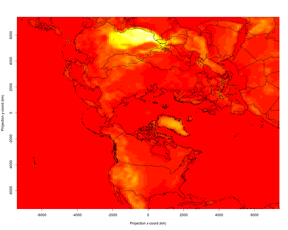
## Make a plot.
image(elev$x.cell.ctr, elev$y.cell.ctr, elev$data[,,1],
      xlab="Projection x-coord (km)", ylab="Projection y-coord (km)",
      zlim=range(elev$data[,,1]), col=heat.colors(15))

## Superimpose national boundaries on the plot
nat.bds <- get.map.lines.M3.proj(file=polar.file, database="world")$coords
lines(nat.bds)


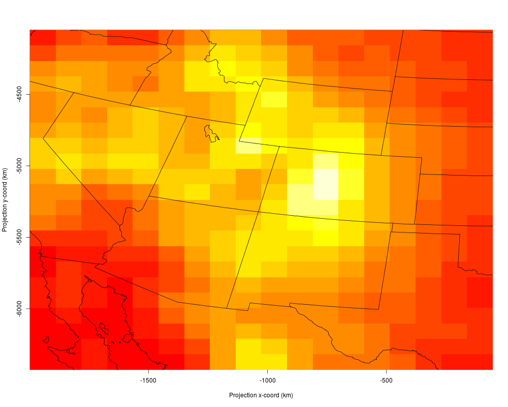
## Subset to a smaller geographic area in southwestern U.S.
subset.elev <- var.subset(elev, llx=-2000, urx=0, lly=-6500, ury=-4000)
## Make a plot of this subset.
image(subset.elev$x.cell.ctr, subset.elev$y.cell.ctr,
      subset.elev$data[,,1], xlab="Projection x-coord (km)",
      ylab="Projection y-coord (km)", zlim=range(subset.elev$data[,,1]),
      col=heat.colors(15))

## Superimpose Mexico, US, and Candadian national borders on the plot,
## along with state borders.
canusamex.bds <- get.map.lines.M3.proj(file=polar.file, "canusamex")$coords
lines(canusamex.bds)

Results


R version 3.3.1 (2016-06-21) -- "Bug in Your Hair"
Copyright (C) 2016 The R Foundation for Statistical Computing
Platform: x86_64-pc-linux-gnu (64-bit)

R is free software and comes with ABSOLUTELY NO WARRANTY.
You are welcome to redistribute it under certain conditions.
Type 'license()' or 'licence()' for distribution details.

R is a collaborative project with many contributors.
Type 'contributors()' for more information and
'citation()' on how to cite R or R packages in publications.

Type 'demo()' for some demos, 'help()' for on-line help, or
'help.start()' for an HTML browser interface to help.
Type 'q()' to quit R.

> library(M3)
Loading required package: ncdf4
Loading required package: rgdal
Loading required package: sp
rgdal: version: 1.1-10, (SVN revision 622)
 Geospatial Data Abstraction Library extensions to R successfully loaded
 Loaded GDAL runtime: GDAL 1.11.3, released 2015/09/16
 Path to GDAL shared files: /usr/share/gdal/1.11
 Loaded PROJ.4 runtime: Rel. 4.9.2, 08 September 2015, [PJ_VERSION: 492]
 Path to PROJ.4 shared files: (autodetected)
 Linking to sp version: 1.2-3 
Loading required package: maps

 # maps v3.1: updated 'world': all lakes moved to separate new #
 # 'lakes' database. Type '?world' or 'news(package="maps")'.  #


Loading required package: mapdata
> png(filename="/home/ddbj/snapshot/RGM3/R_CC/result/M3/get.map.lines.M3.proj.Rd_%03d_medium.png", width=480, height=480)
> ### Name: get.map.lines.M3.proj
> ### Title: Get map lines in the model projection units
> ### Aliases: get.map.lines.M3.proj
> 
> ### ** Examples
> 
> ## Find the path to the demo file.
> polar.file <- system.file("extdata/surfinfo_polar.ncf", package="M3")
> 
> ## Read in the terrain elevation variable.
> elev <- get.M3.var(file=polar.file, var="HT")
Time independent file - reading only time step available.
> ## Make a plot.
> image(elev$x.cell.ctr, elev$y.cell.ctr, elev$data[,,1],
+       xlab="Projection x-coord (km)", ylab="Projection y-coord (km)",
+       zlim=range(elev$data[,,1]), col=heat.colors(15))
> 
> ## Superimpose national boundaries on the plot
> nat.bds <- get.map.lines.M3.proj(file=polar.file, database="world")$coords
> lines(nat.bds)
> 
> 
> ## Subset to a smaller geographic area in southwestern U.S.
> subset.elev <- var.subset(elev, llx=-2000, urx=0, lly=-6500, ury=-4000)
> ## Make a plot of this subset.
> image(subset.elev$x.cell.ctr, subset.elev$y.cell.ctr,
+       subset.elev$data[,,1], xlab="Projection x-coord (km)",
+       ylab="Projection y-coord (km)", zlim=range(subset.elev$data[,,1]),
+       col=heat.colors(15))
> 
> ## Superimpose Mexico, US, and Candadian national borders on the plot,
> ## along with state borders.
> canusamex.bds <- get.map.lines.M3.proj(file=polar.file, "canusamex")$coords
> lines(canusamex.bds)
> 
> 
> 
> 
> 
> dev.off()
null device 
          1 
>