Project coordinates from model units to longitude/latitude

Description

Project coordinates from model units (as specified according to the projection given by a user-designated Models3-formatted file) to longitude/latitude.

Usage

project.M3.to.lonlat(x, y, file, units, ...)

Arguments

Details

This function uses the function project from the package rgdal to project to longitude/latitude given the projection defined by the Models3-formatted file. Package rgdal provides the R interface to GDAL (Geospatial Data Abstraction Library, http://www.gdal.org).

Value

A list containing the elements coords and units. The element coords contains a matrix of coordinates in longitude/latitude. The element units contains the string "deg" to designate that coords is in degrees of longitude/latitude.

Author(s)

Jenise Swall

References

http://www.gdal.org

See Also

project.lonlat.to.M3, project.M3.1.to.M3.2, get.proj.info.M3

Examples

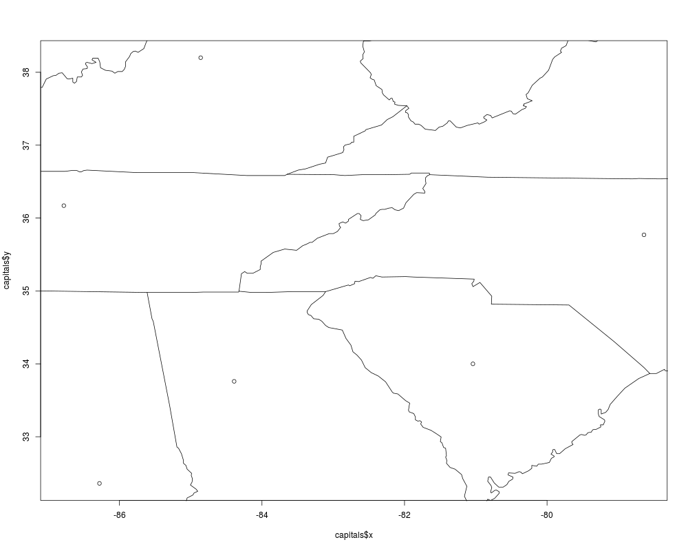
## List of state capital longitudes/latitudes
## (from http://www.xfront.com/us_states).
capitals <- data.frame(x=c(-84.39,-86.28,-81.04,-86.78,-78.64,-84.86),
                       y=c(33.76,32.36,34.00,36.17,35.77,38.20),
                       name=c("Atlanta", "Montgomery", "Columbia",
                                 "Nashville", "Raleigh", "Frankfort")
                        )
## Plot these on a map, with state lines.
plot(capitals$x, capitals$y)
map("state", add=TRUE)

## Now, put these on the same Lambert conic conformal projection used
## in the demo file below.
lcc.file <- system.file("extdata/ozone_lcc.ncf", package="M3")
lcc.capitals <- project.lonlat.to.M3(capitals$x, capitals$y, lcc.file)

## Now, project them back to longitude/latitude, make sure we get the
## same thing we started with.
chk.capitals <- project.M3.to.lonlat(lcc.capitals$coords[,"x"],
                                     lcc.capitals$coords[,"y"],
                                     lcc.file,
                                     units=lcc.capitals$units)
## These differences should be 0 or something very tiny.
summary(capitals[,c("x", "y")] - chk.capitals$coords)

Results

R version 3.3.1 (2016-06-21) -- "Bug in Your Hair"
Copyright (C) 2016 The R Foundation for Statistical Computing
Platform: x86_64-pc-linux-gnu (64-bit)

R is free software and comes with ABSOLUTELY NO WARRANTY.
You are welcome to redistribute it under certain conditions.
Type 'license()' or 'licence()' for distribution details.

R is a collaborative project with many contributors.
Type 'contributors()' for more information and
'citation()' on how to cite R or R packages in publications.

Type 'demo()' for some demos, 'help()' for on-line help, or
'help.start()' for an HTML browser interface to help.
Type 'q()' to quit R.

> library(M3)
Loading required package: ncdf4
Loading required package: rgdal
Loading required package: sp
rgdal: version: 1.1-10, (SVN revision 622)
 Geospatial Data Abstraction Library extensions to R successfully loaded
 Loaded GDAL runtime: GDAL 1.11.3, released 2015/09/16
 Path to GDAL shared files: /usr/share/gdal/1.11
 Loaded PROJ.4 runtime: Rel. 4.9.2, 08 September 2015, [PJ_VERSION: 492]
 Path to PROJ.4 shared files: (autodetected)
 Linking to sp version: 1.2-3 
Loading required package: maps

 # maps v3.1: updated 'world': all lakes moved to separate new #
 # 'lakes' database. Type '?world' or 'news(package="maps")'.  #


Loading required package: mapdata
> png(filename="/home/ddbj/snapshot/RGM3/R_CC/result/M3/project.M3.to.lonlat.Rd_%03d_medium.png", width=480, height=480)
> ### Name: project.M3.to.lonlat
> ### Title: Project coordinates from model units to longitude/latitude
> ### Aliases: project.M3.to.lonlat
> 
> ### ** Examples
> 
> ## List of state capital longitudes/latitudes
> ## (from http://www.xfront.com/us_states).
> capitals <- data.frame(x=c(-84.39,-86.28,-81.04,-86.78,-78.64,-84.86),
+                        y=c(33.76,32.36,34.00,36.17,35.77,38.20),
+                        name=c("Atlanta", "Montgomery", "Columbia",
+                                  "Nashville", "Raleigh", "Frankfort")
+                         )
> ## Plot these on a map, with state lines.
> plot(capitals$x, capitals$y)
> map("state", add=TRUE)
> 
> ## Now, put these on the same Lambert conic conformal projection used
> ## in the demo file below.
> lcc.file <- system.file("extdata/ozone_lcc.ncf", package="M3")
> lcc.capitals <- project.lonlat.to.M3(capitals$x, capitals$y, lcc.file)
> 
> ## Now, project them back to longitude/latitude, make sure we get the
> ## same thing we started with.
> chk.capitals <- project.M3.to.lonlat(lcc.capitals$coords[,"x"],
+                                      lcc.capitals$coords[,"y"],
+                                      lcc.file,
+                                      units=lcc.capitals$units)
> ## These differences should be 0 or something very tiny.
> summary(capitals[,c("x", "y")] - chk.capitals$coords)
       x           y             
 Min.   :0   Min.   :-1.421e-14  
 1st Qu.:0   1st Qu.:-1.066e-14  
 Median :0   Median : 7.105e-15  
 Mean   :0   Mean   : 8.290e-15  
 3rd Qu.:0   3rd Qu.: 2.487e-14  
 Max.   :0   Max.   : 3.553e-14  
> 
> 
> 
> 
> 
> dev.off()
null device 
          1 
>