R Graphical Manual

Browse All

Last data update: 2014.03.03

R: Different generic functions for class MAMS.

plot	R Documentation

Different generic functions for class MAMS.

Description

Generic functions for summarizing an object of class MAMS.

Usage

## S3 method for class 'MAMS'
print(x, digits=max(3, getOption("digits") - 4), ...)

## S3 method for class 'MAMS'
summary(object, digits=max(3, getOption("digits") - 4), ...)

## S3 method for class 'MAMS'
plot(x, col=NULL, pch=NULL, lty=NULL, main=NULL, xlab="Analysis", 
     ylab="Test statistic", ylim=NULL, type=NULL, las=1, ...)

## S3 method for class 'MAMS.sim'
print(x, digits=max(3, getOption("digits") - 4), ...)

## S3 method for class 'MAMS.sim'
summary(object, digits=max(3, getOption("digits") - 4), ...)

## S3 method for class 'MAMS.step_down'
print(x, digits=max(3, getOption("digits") - 4), ...)

## S3 method for class 'MAMS.step_down'
summary(object, digits=max(3, getOption("digits") - 4), ...)

## S3 method for class 'MAMS.step_down'
plot(x, col=NULL, pch=NULL, lty=NULL, main=NULL, xlab="Analysis", 
     ylab="Test statistic", ylim=NULL, type=NULL, bty="n", las=1, ...)

Arguments

`x`	An output object of class MAMS.
`digits`	Number of significant digits to be printed.
`object`	An output object of class MAMS.
`col`	A specification for the default plotting color (default=`NULL`). See `par` for more details.
`pch`	Either an integer specifying a symbol or a single character to be used as the default in plotting points (default=`NULL`). See `par` for more details.
`lty`	A specification for the default line type to be used between analyses (default=`NULL`). Setting to zero supresses ploting of the lines. See `par` for more details.
`main`	An overall title for the plot (default=`NULL`).
`xlab`	A title for the x axis (default=`"Analysis"`).
`ylab`	A title for the y axis (default=`"Test statistic"`).
`ylim`	Numeric vector of length 2, giving the y coordinates range (default=`NULL`).
`type`	Type of plot to be used (default=`NULL`). See `plot` for more details.
`bty`	Should a box be drawn around the legend? The default `"n"` does not draw a box, the alternative option `"o"` does.
`las`	A specification of the axis labeling style. The default `1` ensures the labels are always horizontal. See `?par` for details.
`...`	Further (graphical) arguments to be passed to methods.

Details

print.MAMS produces a summary of an object from class MAMS including boundaries and requires sample size if initially requested.

summary.MAMS produces same output as print.MAMS.

plot.MAMS produces as plot of the boundaries.

print.MAMS.sim produces a summary of an object from class MAMS.sim including type-I-error and expected sample size.

summary.MAMS.sim produces same output as print.MAMS.sim.

print.MAMS.step_down produces a summary of an object from class MAMS including boundaries and requires sample size if initially requested.

summary.MAMS.step_down produces same output as print.step_down_mams.

plot.MAMS.step_down produces a plot of the boundaries. When used with update_mams, pluses indicate observed values of test statistics.

Value

Screen or graphics output.

Author(s)

Thomas Jaki and Dominic Magirr

References

Magirr D, Jaki T, Whitehead J (2012) A generalized Dunnett Test for Multi-arm Multi-stage Clinical Studies with Treatment Selection. Biometrika. 99(2):494-501.

Stallard N, Todd S (2003) Sequential designs for phase III clinical trials incorporating treatment selection. Statistics in Medicine. 22, 689-703.

Magirr D, Stallard N, Jaki T (2014) Flexible sequential designs for multi-arm clinical trials. Statistics in Medicine. Published online.

Examples


# 2-stage design with triangular boundaries
res <- mams(K=4, J=2, alpha=0.05, power=0.9, r=1:2, r0=1:2, p=0.65 , p0=0.55, 
            u.shape="triangular", l.shape="triangular", nstart=30)

print(res)
summary(res)
plot(res)

res <- mams.sim(nsim=10000, nMat=matrix(c(44, 88), nrow=2, ncol=5), u=c(3.068, 2.169),
                l=c(0.000, 2.169), pv=c(0.65, 0.55, 0.55, 0.55), ptest=c(1:2, 4))

print(res)

# 2-stage 3-treatments versus control design, all promising treatments are selected:
res <- step_down_mams(nMat=matrix(c(10, 20), nrow=2, ncol=4), 
                      alpha_star=c(0.01, 0.05), lb=0, 
                      selection="all_promising")

print(res)
summary(res)
plot(res)

Results


R version 3.3.1 (2016-06-21) -- "Bug in Your Hair"
Copyright (C) 2016 The R Foundation for Statistical Computing
Platform: x86_64-pc-linux-gnu (64-bit)

R is free software and comes with ABSOLUTELY NO WARRANTY.
You are welcome to redistribute it under certain conditions.
Type 'license()' or 'licence()' for distribution details.

R is a collaborative project with many contributors.
Type 'contributors()' for more information and
'citation()' on how to cite R or R packages in publications.

Type 'demo()' for some demos, 'help()' for on-line help, or
'help.start()' for an HTML browser interface to help.
Type 'q()' to quit R.

> library(MAMS)
Loading required package: mvtnorm
 **********   MAMS Version 0.9********** 

Type MAMSNews() to see new features/changes/bug fixes.

> png(filename="/home/ddbj/snapshot/RGM3/R_CC/result/MAMS/generic.Rd_%03d_medium.png", width=480, height=480)
> ### Name: plot
> ### Title: Different generic functions for class MAMS.
> ### Aliases: plot.MAMS print.MAMS summary.MAMS print.MAMS.sim
> ###   summary.MAMS.sim print.MAMS.step_down summary.MAMS.step_down
> ###   plot.MAMS.step_down
> ### Keywords: classes
> 
> ### ** Examples
> 
> ## No test: 
> # 2-stage design with triangular boundaries
> res <- mams(K=4, J=2, alpha=0.05, power=0.9, r=1:2, r0=1:2, p=0.65 , p0=0.55, 
+             u.shape="triangular", l.shape="triangular", nstart=30)
> 
> print(res)
Design parameters for a 2 stage trial with 4 treatments

                                            Stage 1 Stage 2
Cumulative sample size per stage (control):      50     100
Cumulative sample size per stage (active):       50     100

Maximum total sample size:  500 

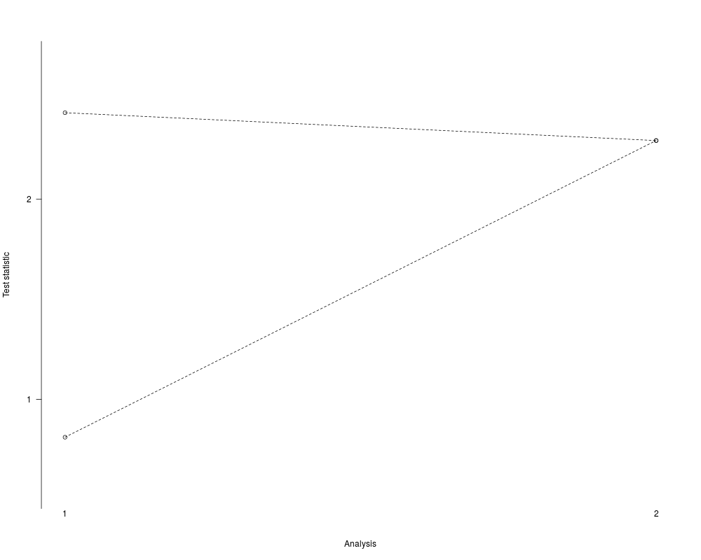
             Stage 1 Stage 2
Upper bound:   2.432   2.293
Lower bound:   0.811   2.293
> summary(res)
Design parameters for a 2 stage trial with 4 treatments

                                            Stage 1 Stage 2
Cumulative sample size per stage (control):      50     100
Cumulative sample size per stage (active):       50     100

Maximum total sample size:  500 

             Stage 1 Stage 2
Upper bound:   2.432   2.293
Lower bound:   0.811   2.293
> plot(res)
> ## End(No test)
> res <- mams.sim(nsim=10000, nMat=matrix(c(44, 88), nrow=2, ncol=5), u=c(3.068, 2.169),
+                 l=c(0.000, 2.169), pv=c(0.65, 0.55, 0.55, 0.55), ptest=c(1:2, 4))
> 
> print(res)
Simulated error rates based on 10000 simulations

                                                          
Prop. rejecting at least 1 hypothesis:               0.929
Prop. rejecting first hypothesis (Z_1>Z_2,...,Z_K)   0.904
Prop. rejecting hypotheses 1 or 2 or 4:              0.926
Expected sample size:                              346.328
> 
> # 2-stage 3-treatments versus control design, all promising treatments are selected:
> res <- step_down_mams(nMat=matrix(c(10, 20), nrow=2, ncol=4), 
+                       alpha_star=c(0.01, 0.05), lb=0, 
+                       selection="all_promising")
> 
> print(res)
Design parameters for a 2 stage trial with 3 treatments

                                                  Stage 1 Stage 2
Cumulative sample size  (control):                     10      20
Cumulative sample size per stage (treatment  1 ):      10      20
Cumulative sample size per stage (treatment  2 ):      10      20
Cumulative sample size per stage (treatment  3 ):      10      20

Maximum total sample size:  80 


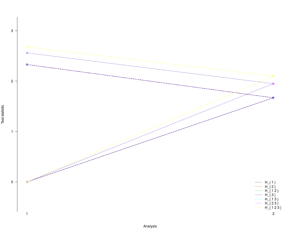
Intersection hypothesis H_{ 1 }: 

                  Stage 1 Stage 2
Conditional error    0.01    0.05
Upper boundary       2.33    1.67
Lower boundary       0.00    1.67

Intersection hypothesis H_{ 2 }: 

                  Stage 1 Stage 2
Conditional error    0.01    0.05
Upper boundary       2.33    1.67
Lower boundary       0.00    1.67

Intersection hypothesis H_{ 1 2 }: 

                  Stage 1 Stage 2
Conditional error    0.01    0.05
Upper boundary       2.56    1.95
Lower boundary       0.00    1.95

Intersection hypothesis H_{ 3 }: 

                  Stage 1 Stage 2
Conditional error    0.01    0.05
Upper boundary       2.33    1.67
Lower boundary       0.00    1.67

Intersection hypothesis H_{ 1 3 }: 

                  Stage 1 Stage 2
Conditional error    0.01    0.05
Upper boundary       2.56    1.95
Lower boundary       0.00    1.95

Intersection hypothesis H_{ 2 3 }: 

                  Stage 1 Stage 2
Conditional error    0.01    0.05
Upper boundary       2.56    1.95
Lower boundary       0.00    1.95

Intersection hypothesis H_{ 1 2 3 }: 

                  Stage 1 Stage 2
Conditional error    0.01    0.05
Upper boundary       2.68    2.10
Lower boundary       0.00    2.10
> summary(res)
Design parameters for a 2 stage trial with 3 treatments

                                                  Stage 1 Stage 2
Cumulative sample size  (control):                     10      20
Cumulative sample size per stage (treatment  1 ):      10      20
Cumulative sample size per stage (treatment  2 ):      10      20
Cumulative sample size per stage (treatment  3 ):      10      20

Maximum total sample size:  80 


Intersection hypothesis H_{ 1 }: 

                  Stage 1 Stage 2
Conditional error    0.01    0.05
Upper boundary       2.33    1.67
Lower boundary       0.00    1.67

Intersection hypothesis H_{ 2 }: 

                  Stage 1 Stage 2
Conditional error    0.01    0.05
Upper boundary       2.33    1.67
Lower boundary       0.00    1.67

Intersection hypothesis H_{ 1 2 }: 

                  Stage 1 Stage 2
Conditional error    0.01    0.05
Upper boundary       2.56    1.95
Lower boundary       0.00    1.95

Intersection hypothesis H_{ 3 }: 

                  Stage 1 Stage 2
Conditional error    0.01    0.05
Upper boundary       2.33    1.67
Lower boundary       0.00    1.67

Intersection hypothesis H_{ 1 3 }: 

                  Stage 1 Stage 2
Conditional error    0.01    0.05
Upper boundary       2.56    1.95
Lower boundary       0.00    1.95

Intersection hypothesis H_{ 2 3 }: 

                  Stage 1 Stage 2
Conditional error    0.01    0.05
Upper boundary       2.56    1.95
Lower boundary       0.00    1.95

Intersection hypothesis H_{ 1 2 3 }: 

                  Stage 1 Stage 2
Conditional error    0.01    0.05
Upper boundary       2.68    2.10
Lower boundary       0.00    2.10
> plot(res)
> 
> 
> 
> 
> 
> 
> dev.off()
null device 
          1 
>