R Graphical Manual

Browse All

Last data update: 2014.03.03

R: Kaplan-Meier Estimate

WKME	R Documentation

Kaplan-Meier Estimate

Description

Computes the weighted Kaplan-Meier estimate over some time points with optional confidence intervals.

Usage

WKME(x,ub,lb=0,time=NULL,boot=NULL,REP=1000)

Arguments

`x`	A list of `m` samples. Each element is an `n` by `2` matrix whose second column is an indicator of whether the time in column 1 is observed (1) or censored (0).
`lb,ub`	Lower and upper bounds of the integral of the MAMSE criterion.
`time`	A vector of times at which to compute the Kaplan-Meier estimate.
`boot`	When NULL, bootstrap confidence intervals are not generated. Otherwise must be a number in (0,1) corresponding to the coverage probability of the bootstrap intervals to be built.
`REP`	When bootstrap is used, controls the number of pseudo-sample to generate.

Details

This function calculates the weighted Kaplan-Meier estimate and can provide pointwise bootstrap confidence intervals.

Value

List of elements:

`x`	Sorted list of the times (observed and censored) from each samples
`weight`	The size of the jump that the Kaplan-Meier estimate allocates to each time in `x`.
`time`	Vector of time points where the function is evaluated.
`kme`	The Kaplan-Meier estimate for Population 1 evaluated at `time`.
`kmeCI`	Pointwise bootstrap confidence interval for `kme`.
`wkme`	The weighted Kaplan-Meier estimate evaluated at `time`.
`wkmeCI`	Pointwise bootstrap confidence interval for `wkme`.

References

J.-F. Plante (2007). Adaptive Likelihood Weights and Mixtures of Empirical Distributions. Unpublished doctoral dissertation, University of British Columbia.

J.-F. Plante (2009). About an adaptively weighted Kaplan-Meier estimate. Lifetime Data Analysis, 15, 295-315.

Examples

set.seed(2009)
x=list(
  cbind(rexp(20),sample(c(0,1),20,replace=TRUE)),
  cbind(rexp(50),sample(c(0,1),50,replace=TRUE)),
  cbind(rexp(100),sample(c(0,1),100,replace=TRUE))
)

allx=pmin(1,c(x[[1]][x[[1]][,2]==1,1],x[[2]][x[[2]][,2]==1,1],
   x[[3]][x[[3]][,2]==1,1]))
K=WKME(x,1,time=sort(unique(c(0,1,allx,allx-.0001))),boot=.9,REP=100)
# Only 100 bootstrap repetitions were used to get a fast enough
# calculation on a CRAN check.

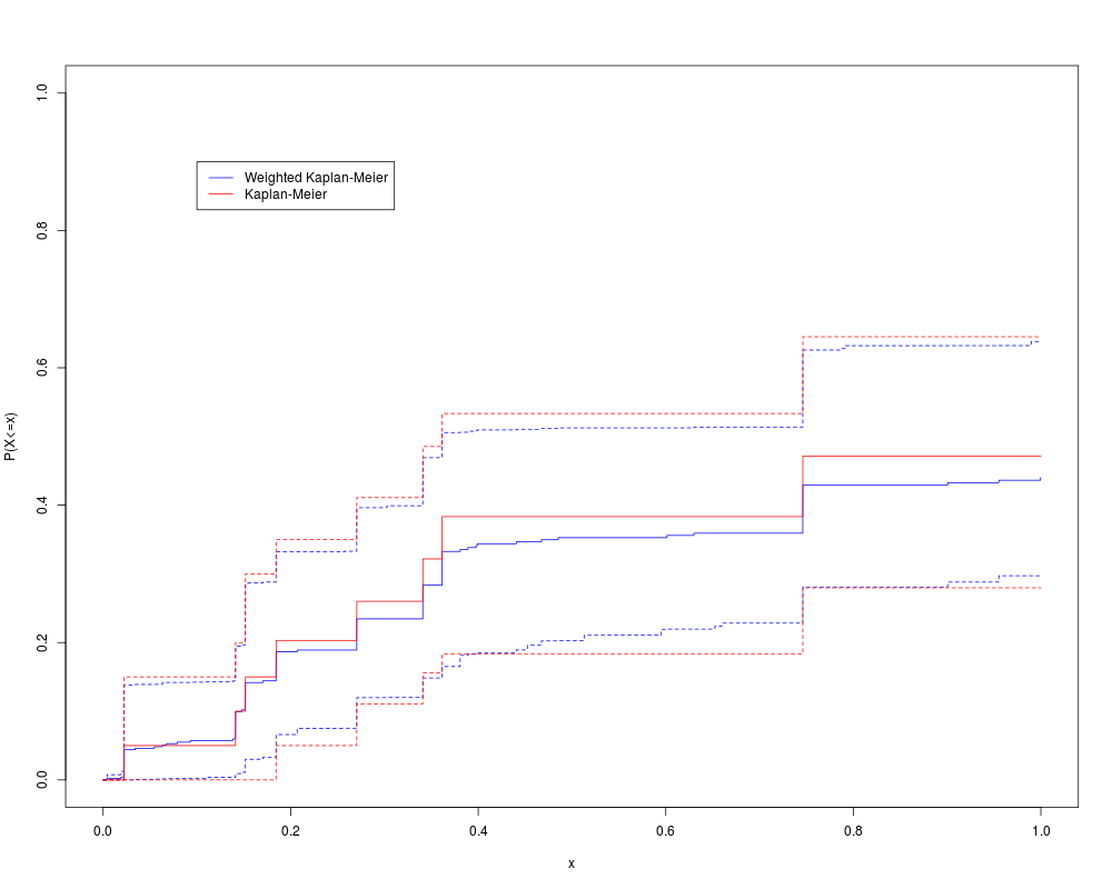
plot(K$time,K$wkme,type='l',col="blue",xlab="x",
   ylab="P(X<=x)",ylim=c(0,1))
lines(K$time,K$kme[,1],col="red")

lines(K$time,K$wkmeCI[1,],lty=2,col="blue")
lines(K$time,K$wkmeCI[2,],lty=2,col="blue")

lines(K$time,K$kmeCI[1,],lty=2,col="red")
lines(K$time,K$kmeCI[2,],lty=2,col="red")
legend(.1,.9,c("Weighted Kaplan-Meier","Kaplan-Meier"),
   col=c("blue","red"),lty=c(1,1))

Results


R version 3.3.1 (2016-06-21) -- "Bug in Your Hair"
Copyright (C) 2016 The R Foundation for Statistical Computing
Platform: x86_64-pc-linux-gnu (64-bit)

R is free software and comes with ABSOLUTELY NO WARRANTY.
You are welcome to redistribute it under certain conditions.
Type 'license()' or 'licence()' for distribution details.

R is a collaborative project with many contributors.
Type 'contributors()' for more information and
'citation()' on how to cite R or R packages in publications.

Type 'demo()' for some demos, 'help()' for on-line help, or
'help.start()' for an HTML browser interface to help.
Type 'q()' to quit R.

> library(MAMSE)
> png(filename="/home/ddbj/snapshot/RGM3/R_CC/result/MAMSE/WKME.Rd_%03d_medium.png", width=480, height=480)
> ### Name: WKME
> ### Title: Kaplan-Meier Estimate
> ### Aliases: WKME
> ### Keywords: nonparametric survival
> 
> ### ** Examples
> 
> set.seed(2009)
> x=list(
+   cbind(rexp(20),sample(c(0,1),20,replace=TRUE)),
+   cbind(rexp(50),sample(c(0,1),50,replace=TRUE)),
+   cbind(rexp(100),sample(c(0,1),100,replace=TRUE))
+ )
> 
> allx=pmin(1,c(x[[1]][x[[1]][,2]==1,1],x[[2]][x[[2]][,2]==1,1],
+    x[[3]][x[[3]][,2]==1,1]))
> K=WKME(x,1,time=sort(unique(c(0,1,allx,allx-.0001))),boot=.9,REP=100)
Warning message:
In MAMSEsurvpo(Z, lb = lb, ub = ub) :
  Too few data points from Population 1 fall in the interval of interest.
> # Only 100 bootstrap repetitions were used to get a fast enough
> # calculation on a CRAN check.
> 
> plot(K$time,K$wkme,type='l',col="blue",xlab="x",
+    ylab="P(X<=x)",ylim=c(0,1))
> lines(K$time,K$kme[,1],col="red")
> 
> lines(K$time,K$wkmeCI[1,],lty=2,col="blue")
> lines(K$time,K$wkmeCI[2,],lty=2,col="blue")
> 
> lines(K$time,K$kmeCI[1,],lty=2,col="red")
> lines(K$time,K$kmeCI[2,],lty=2,col="red")
> legend(.1,.9,c("Weighted Kaplan-Meier","Kaplan-Meier"),
+    col=c("blue","red"),lty=c(1,1))
> 
> 
> 
> 
> 
> 
> dev.off()
null device 
          1 
>