Spatial bias detection

Description

This function detects spatial bias on array CGH.

Usage

## S3 method for class 'arrayCGH'
detectSB(arrayCGH, variable, proportionup=0.25,
proportiondown,type="up", thresholdup=0.2, thresholddown=0.2, ... ) 

Arguments

Details

You must run the arrayTrend and nem function before detecting spatial bias: the arrayTrend computes a spatial trend and the nem function performs a classification with spatial constraints defining different zones on the array. Based on those results, spatial bias is detected.

Value

An object of class arrayCGH with the following added information in the data.frame attribute arrayValues:

Note

People interested in tools for array-CGH analysis can visit our web-page: http://bioinfo.curie.fr.

Author(s)

Philippe Hupé, Philippe.Hupe@.curie.fr.

References

P. Neuvial, P. Hupé, I. Brito, S. Liva, E. Manié, C. Brennetot, A. Aurias, F. Radvanyi, and E. Barillot. Spatial normalization of array-CGH data. BMC Bioinformatics, 7(1):264. May 2006.

See Also

arrayTrend, nem

Examples

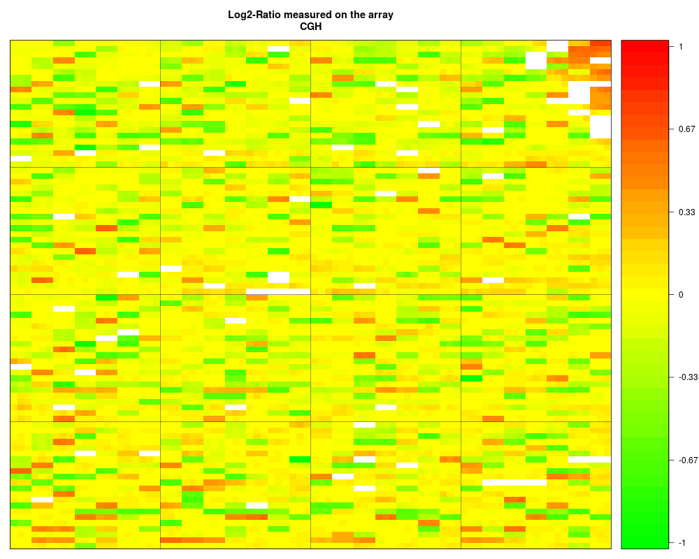
data(spatial)  ## arrays with local spatial effects

## Plot of LogRatio measured on the array CGH
arrayPlot(edge,"LogRatio", main="Log2-Ratio measured on the array
CGH", zlim=c(-1,1), bar="v", mediancenter=TRUE) 

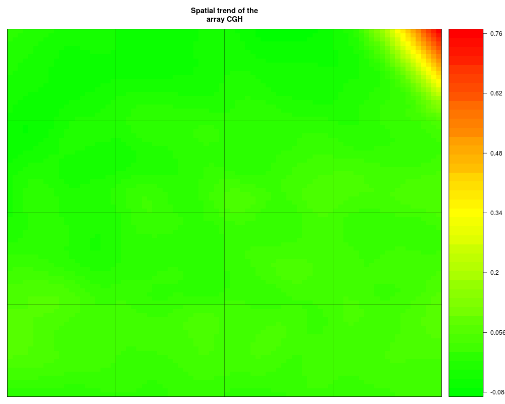
## Spatial trend of the scaled log-ratios (the variable "ScaledLogRatio"
## equals to the log-ratio minus the median value of the corresponding
## chromosome arm)

edgeTrend <- arrayTrend(edge, variable="ScaledLogRatio",
span=0.03, degree=1, iterations=3, family="symmetric")   
arrayPlot(edgeTrend, variable="Trend", main="Spatial trend of the
array CGH", bar="v")  

## Not run: 
## Classification with spatial constraint of the spatial trend
edgeNem <- nem(edgeTrend, variable="Trend")
arrayPlot(edgeNem, variable="ZoneNem", main="Spatial zones identified
by nem", bar="v") 

# Detection of spatial bias
edgeDet <- detectSB(edgeNem, variable="LogRatio", proportionup=0.25,type="up", thresholdup=0.15) 
arrayPlot(edgeDet, variable="SB", main="Zone of spatial bias in red", bar="v")

# CGH profile 
plot(LogRatio ~ PosOrder, data=edgeDet$arrayValues,
col=c("black","red")[as.factor(SB)], pch=20, main="CGH profile: spots
located in spatial bias are in red")  

## End(Not run)

Results

R version 3.3.1 (2016-06-21) -- "Bug in Your Hair"
Copyright (C) 2016 The R Foundation for Statistical Computing
Platform: x86_64-pc-linux-gnu (64-bit)

R is free software and comes with ABSOLUTELY NO WARRANTY.
You are welcome to redistribute it under certain conditions.
Type 'license()' or 'licence()' for distribution details.

R is a collaborative project with many contributors.
Type 'contributors()' for more information and
'citation()' on how to cite R or R packages in publications.

Type 'demo()' for some demos, 'help()' for on-line help, or
'help.start()' for an HTML browser interface to help.
Type 'q()' to quit R.

> library(MANOR)
Loading required package: GLAD

######################################################################################

Have fun with GLAD

For smoothing it is possible to use either
the AWS algorithm (Polzehl and Spokoiny, 2002,
or the HaarSeg algorithm (Ben-Yaacov and Eldar, Bioinformatics,  2008,

If you use the package with AWS, please cite:
Hupe et al. (Bioinformatics, 2004, and Polzehl and Spokoiny (2002,

If you use the package with HaarSeg, please cite:
Hupe et al. (Bioinformatics, 2004, and (Ben-Yaacov and Eldar, Bioinformatics, 2008,

For fast computation it is recommanded to use
the daglad function with smoothfunc=haarseg

######################################################################################

New options are available in daglad: see help for details.


Attaching package: 'MANOR'

The following object is masked from 'package:base':

    norm

> png(filename="/home/ddbj/snapshot/RGM3/R_BC/result/MANOR/detectSB.Rd_%03d_medium.png", width=480, height=480)
> ### Name: detectSB
> ### Title: Spatial bias detection
> ### Aliases: detectSB detectSB.default detectSB.arrayCGH
> ### Keywords: models spatial
> 
> ### ** Examples
> 
> data(spatial)  ## arrays with local spatial effects
> 
> ## Plot of LogRatio measured on the array CGH
> arrayPlot(edge,"LogRatio", main="Log2-Ratio measured on the array
+ CGH", zlim=c(-1,1), bar="v", mediancenter=TRUE) 
> 
> ## Spatial trend of the scaled log-ratios (the variable "ScaledLogRatio"
> ## equals to the log-ratio minus the median value of the corresponding
> ## chromosome arm)
> 
> edgeTrend <- arrayTrend(edge, variable="ScaledLogRatio",
+ span=0.03, degree=1, iterations=3, family="symmetric")   
> arrayPlot(edgeTrend, variable="Trend", main="Spatial trend of the
+ array CGH", bar="v")  
> 
> ## Not run: 
> ##D ## Classification with spatial constraint of the spatial trend
> ##D edgeNem <- nem(edgeTrend, variable="Trend")
> ##D arrayPlot(edgeNem, variable="ZoneNem", main="Spatial zones identified
> ##D by nem", bar="v") 
> ##D 
> ##D # Detection of spatial bias
> ##D edgeDet <- detectSB(edgeNem, variable="LogRatio", proportionup=0.25,type="up", thresholdup=0.15) 
> ##D arrayPlot(edgeDet, variable="SB", main="Zone of spatial bias in red", bar="v")
> ##D 
> ##D # CGH profile 
> ##D plot(LogRatio ~ PosOrder, data=edgeDet$arrayValues,
> ##D col=c("black","red")[as.factor(SB)], pch=20, main="CGH profile: spots
> ##D located in spatial bias are in red")  
> ## End(Not run)
> 
> 
> 
> 
> 
> dev.off()
null device 
          1 
>