Normalize an object of type arrayCGH

Description

Normalize an object of type arrayCGH using a list of criteria specified as (temporary or permanent) flags. If a replicate identifier (clone name) is provided, a single target value is computed for all the replicates.

The normalization coefficient is computed as a function, and is applied to all good quality spots of the array.

Usage

  ## S3 method for class 'arrayCGH'
norm(arrayCGH, flag.list=NULL, var="LogRatio", printTime=FALSE, FUN=median, ...)

Arguments

Details

The two flag types are treated differently : - permanent flags detect poor quality spots, which are removed from further analysis - temporary flags detect good quality spots that would bias the normalization coefficient if they were not excluded from its computation, e.g. amplicons or sexual chromosomes. Thus they are not taken into account for the computation of the coefficient, but at the end of the analysis they are normalized as any good quality spots of the array.

The normalization coefficient is computed as a function (e.g. mean or median) of the target value (e.g. log-ratios); it is then applied to all good quality spots (including temporary flags), i.e. substracted from each target value.

If clone level information is available (i.e. if arrayCGH$cloneValues is not null), a normalized mean target value and basic statistics (such as the number of replicates per clone) are calculated for each clone.

Value

an object of type arrayCGH

Note

People interested in tools for array-CGH analysis can visit our web-page: http://bioinfo.curie.fr.

Author(s)

Pierre Neuvial, manor@curie.fr.

References

P. Neuvial, P. Hupé, I. Brito, S. Liva, E. Manié, C. Brennetot, A. Aurias, F. Radvanyi, and E. Barillot. Spatial normalization of array-CGH data. BMC Bioinformatics, 7(1):264. May 2006.

See Also

flag

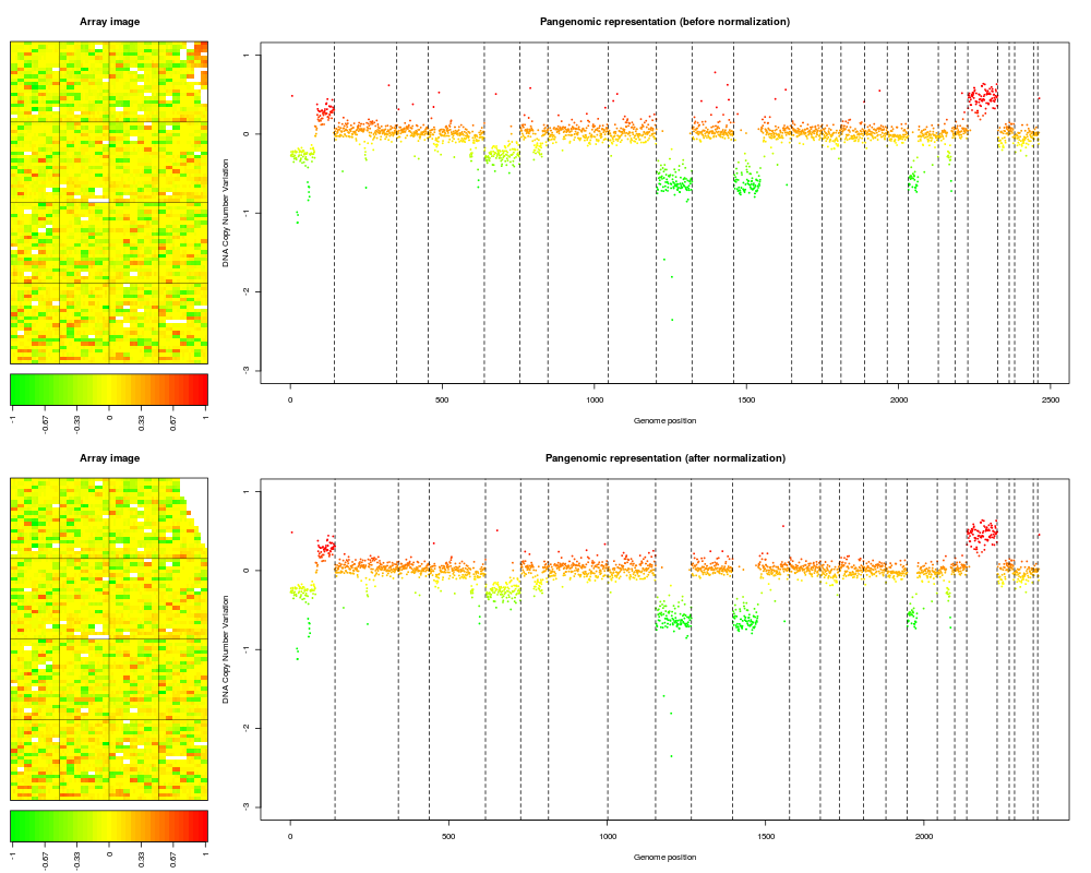
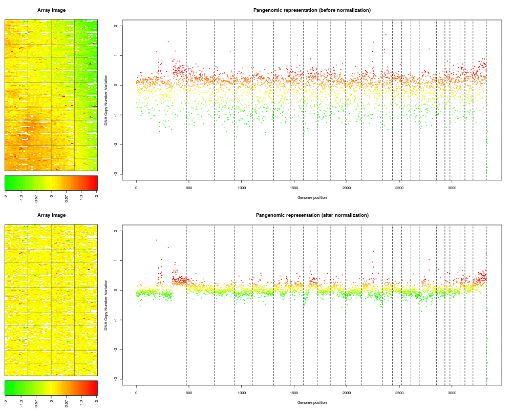
Examples

data(spatial)
data(flags)

### 'edge': local spatial bias
## define a list of flags to be applied
flag.list1 <- list(spatial=local.spatial.flag, spot=spot.corr.flag,
ref.snr=ref.snr.flag, dapi.snr=dapi.snr.flag, rep=rep.flag,
unique=unique.flag) 
flag.list1$spatial$args <- alist(var="ScaledLogRatio", by.var=NULL,
nk=5, prop=0.25, thr=0.15, beta=1, family="symmetric") 
flag.list1$spot$args <- alist(var="SpotFlag")
flag.list1$spot$char <- "O"
flag.list1$spot$label <- "Image analysis"

## normalize arrayCGH
## Not run: edge.norm <- norm(edge, flag.list=flag.list1,
var="LogRatio", FUN=median, na.rm=TRUE)
## End(Not run) 
print(edge.norm$flags) ## spot-level flag summary (computed by flag.summary)

## aggregate arrayCGH without normalization
edge.nonorm <- norm(edge, flag.list=NULL, var="LogRatio",
FUN=median, na.rm=TRUE)  

## sort genomic informations 
edge.norm <- sort(edge.norm, position.var="PosOrder")
edge.nonorm <- sort(edge.nonorm, position.var="PosOrder")

## plot genomic profiles
layout(matrix(c(1,2,4,5,3,3,6,6), 4,2),width=c(1, 4), height=c(6,1,6,1))
report.plot(edge.nonorm, chrLim="LimitChr", layout=FALSE,
main="Pangenomic representation (before normalization)", zlim=c(-1,1),
ylim=c(-3,1))  
report.plot(edge.norm, chrLim="LimitChr", layout=FALSE,
main="Pangenomic representation (after normalization)", zlim=c(-1,1),
ylim=c(-3,1)) 

### 'gradient': global array Trend
## define a list of flags to be applied
flag.list2 <- list(
  spot=spot.flag, global.spatial=global.spatial.flag, SNR=SNR.flag,
  val.mark=val.mark.flag, position=position.flag, unique=unique.flag,
  amplicon=amplicon.flag, replicate=replicate.flag,
  chromosome=chromosome.flag)

## normalize arrayCGH
## Not run: gradient.norm <- norm(gradient, flag.list=flag.list2, var="LogRatio", FUN=median, na.rm=TRUE) 
## aggregate arrayCGH without normalization
gradient.nonorm <- norm(gradient, flag.list=NULL, var="LogRatio", FUN=median, na.rm=TRUE) 

## sort genomic informations 
gradient.norm <- sort(gradient.norm)
gradient.nonorm <- sort(gradient.nonorm)

## plot genomic profiles
layout(matrix(c(1,2,4,5,3,3,6,6), 4,2),width=c(1, 4), height=c(6,1,6,1))
report.plot(gradient.nonorm, chrLim="LimitChr", layout=FALSE,
main="Pangenomic representation (before normalization)", zlim=c(-2,2),
ylim=c(-3,2)) 
report.plot(gradient.norm, chrLim="LimitChr", layout=FALSE,
main="Pangenomic representation (after normalization)", zlim=c(-2,2),
ylim=c(-3,2)) 

Results

R version 3.3.1 (2016-06-21) -- "Bug in Your Hair"
Copyright (C) 2016 The R Foundation for Statistical Computing
Platform: x86_64-pc-linux-gnu (64-bit)

R is free software and comes with ABSOLUTELY NO WARRANTY.
You are welcome to redistribute it under certain conditions.
Type 'license()' or 'licence()' for distribution details.

R is a collaborative project with many contributors.
Type 'contributors()' for more information and
'citation()' on how to cite R or R packages in publications.

Type 'demo()' for some demos, 'help()' for on-line help, or
'help.start()' for an HTML browser interface to help.
Type 'q()' to quit R.

> library(MANOR)
Loading required package: GLAD

######################################################################################

Have fun with GLAD

For smoothing it is possible to use either
the AWS algorithm (Polzehl and Spokoiny, 2002,
or the HaarSeg algorithm (Ben-Yaacov and Eldar, Bioinformatics,  2008,

If you use the package with AWS, please cite:
Hupe et al. (Bioinformatics, 2004, and Polzehl and Spokoiny (2002,

If you use the package with HaarSeg, please cite:
Hupe et al. (Bioinformatics, 2004, and (Ben-Yaacov and Eldar, Bioinformatics, 2008,

For fast computation it is recommanded to use
the daglad function with smoothfunc=haarseg

######################################################################################

New options are available in daglad: see help for details.


Attaching package: 'MANOR'

The following object is masked from 'package:base':

    norm

> png(filename="/home/ddbj/snapshot/RGM3/R_BC/result/MANOR/norm.Rd_%03d_medium.png", width=480, height=480)
> ### Name: norm
> ### Title: Normalize an object of type arrayCGH
> ### Aliases: norm.arrayCGH norm MANOR manor
> ### Keywords: models
> 
> ### ** Examples
> 
> data(spatial)
> data(flags)
> 
> ### 'edge': local spatial bias
> ## define a list of flags to be applied
> flag.list1 <- list(spatial=local.spatial.flag, spot=spot.corr.flag,
+ ref.snr=ref.snr.flag, dapi.snr=dapi.snr.flag, rep=rep.flag,
+ unique=unique.flag) 
> flag.list1$spatial$args <- alist(var="ScaledLogRatio", by.var=NULL,
+ nk=5, prop=0.25, thr=0.15, beta=1, family="symmetric") 
> flag.list1$spot$args <- alist(var="SpotFlag")
> flag.list1$spot$char <- "O"
> flag.list1$spot$label <- "Image analysis"
> 
> ## normalize arrayCGH
> ## Not run: 
> ##D edge.norm <- norm(edge, flag.list=flag.list1,
> ##D var="LogRatio", FUN=median, na.rm=TRUE)
> ## End(Not run) 
> print(edge.norm$flags) ## spot-level flag summary (computed by flag.summary)
  char                            label  arg count
1    S                       Local bias   NA   127
2    O                   Image analysis   NA    37
3    B  Low signal to noise ratio (Ref) 1.25    19
4    D Low signal to noise ratio (Dapi) 1.25    85
5    E       Poor replicate consistency 0.10     0
6    U                          Singlet   NA     8
7   OK                      not flagged   NA  7116
> 
> ## aggregate arrayCGH without normalization
> edge.nonorm <- norm(edge, flag.list=NULL, var="LogRatio",
+ FUN=median, na.rm=TRUE)  
> 
> ## sort genomic informations 
> edge.norm <- sort(edge.norm, position.var="PosOrder")
> edge.nonorm <- sort(edge.nonorm, position.var="PosOrder")
> 
> ## plot genomic profiles
> layout(matrix(c(1,2,4,5,3,3,6,6), 4,2),width=c(1, 4), height=c(6,1,6,1))
> report.plot(edge.nonorm, chrLim="LimitChr", layout=FALSE,
+ main="Pangenomic representation (before normalization)", zlim=c(-1,1),
+ ylim=c(-3,1))  
> report.plot(edge.norm, chrLim="LimitChr", layout=FALSE,
+ main="Pangenomic representation (after normalization)", zlim=c(-1,1),
+ ylim=c(-3,1)) 
> 
> ### 'gradient': global array Trend
> ## define a list of flags to be applied
> flag.list2 <- list(
+   spot=spot.flag, global.spatial=global.spatial.flag, SNR=SNR.flag,
+   val.mark=val.mark.flag, position=position.flag, unique=unique.flag,
+   amplicon=amplicon.flag, replicate=replicate.flag,
+   chromosome=chromosome.flag)
> 
> ## normalize arrayCGH
> ## Not run: gradient.norm <- norm(gradient, flag.list=flag.list2, var="LogRatio", FUN=median, na.rm=TRUE) 
> ## aggregate arrayCGH without normalization
> gradient.nonorm <- norm(gradient, flag.list=NULL, var="LogRatio", FUN=median, na.rm=TRUE) 
> 
> ## sort genomic informations 
> gradient.norm <- sort(gradient.norm)
> gradient.nonorm <- sort(gradient.nonorm)
> 
> ## plot genomic profiles
> layout(matrix(c(1,2,4,5,3,3,6,6), 4,2),width=c(1, 4), height=c(6,1,6,1))
> report.plot(gradient.nonorm, chrLim="LimitChr", layout=FALSE,
+ main="Pangenomic representation (before normalization)", zlim=c(-2,2),
+ ylim=c(-3,2)) 
> report.plot(gradient.norm, chrLim="LimitChr", layout=FALSE,
+ main="Pangenomic representation (after normalization)", zlim=c(-2,2),
+ ylim=c(-3,2)) 
> 
> 
> 
> 
> 
> dev.off()
null device 
          1 
>